Appendix B · Mathematical Formalization
~190 min left · 47,318 words
Appendix B · Mathematical Formalization
This appendix provides mathematical formalization for concepts expressed in natural language in the main text. It is optional: skipping it does not affect understanding of Lucidosophy. But for those who, like Logonaut, love precise formulations, this appendix reveals the mathematical structures behind Lucidosophy’s concepts, and their philosophical implications.
The appendix has five parts. Part I (B.1) gives the core concepts mathematical definitions and is the ground for everything after it. Part II (B.2 to B.6) formalizes Pattern’s four fundamental modes (dissipation, gradient, selection, feedback) and builds an information-theoretic model of obscuration. Part III (B.7 to B.11) works where Pattern reaches the edge of Mystery: experience, finitude, cognitive limits, emergence, and ethical interaction. Part IV (B.12 to B.17) is the mathematics of lucidity itself: the lucidity product, dual-face optimality, the master equation, multi-agent dynamics and collective lucidity, and the consequences at cosmic scale. Part V (B.18) turns the first four parts into exercises. A physics audit at the end of the appendix records what the framework borrows from physics and what it sets aside. Sections B.2 to B.17 follow the same order: setup, results and proofs, worked example, interpretation, insights, and last “Scope and limits,” which gathers the section’s caveats. The interpretation opens by restating the section’s results in everyday terms; the insights state what those results mean for thought and practice, the first two readable without any formula and the rest citing their mathematical source, and every one keeps the conditions the result carries; B.1’s interpretation and insights close that section. A section with no results or no example omits that part.
Definitions, assumptions, and results are numbered consecutively within each section: “Theorem B.12.6” is the sixth numbered item in B.12. The appendix and the main text cite these items by that number.
Reading guide. This appendix is modular. If you know basic calculus and probability: read everything. If you know algebra but not calculus: skip B.3, B.5, B.12–B.15; the remaining sections use only set theory, logic, and discrete mathematics. If you are a philosophy reader with no math background: read B.1 (the ontological foundation), B.9 (Gödel and cognitive limits), B.11 (game theory of ethics), and B.18 (practice exercises). These sections are written to be accessible with minimal mathematical prerequisites.
A note on content types. This appendix contains three kinds of material, and knowing which kind you are reading matters:
Independent mathematical results: constructions and proofs that hold on their own terms within the chosen formalism (e.g., the gradient theorem in B.12, the game-theoretic equilibria in B.11). These are genuine mathematical derivations.
Formal models: mathematical structures that operationalize philosophical claims by giving them precise definitions and exploring their consequences (e.g., the five-tuple model of Reality in B.1, the lucidity product \(\mathcal{M} = \lambda \cdot \xi\) in B.1.4 and B.12). These are modeling choices: illuminating and disciplined, but not uniquely forced by the philosophy.
Symbolic restatements: translations of main-text propositions into formal notation, making their logical structure explicit without adding new mathematical content.
All three are valuable, but they differ in what they demonstrate. The first proves; the second models; the third clarifies. On the page, numbered Definitions and Assumptions are modeling choices and belong to the second kind; numbered Theorems, Propositions, and Corollaries are results that hold within the chosen formalism and belong to the first, proved either here or in the standard literature. An item whose heading names a main-text number (such as T7) is the formal version of a main-text claim and reads alongside it. Of each unnumbered derivation or reading, ask first which kind it is.
Notation
The table lists the symbols that recur across the appendix and where each is defined. A few letters take another meaning in a single section (for instance \(\beta\) in B.5 and \(W\) in B.15); there the section’s own note governs.
| Symbol | Meaning | Defined in |
|---|---|---|
| Symbol | Meaning | Defined in |
\(\Omega\) |
the totality of Reality, the sample space | Definition B.1.1 |
| \(\mu\), \(\tau\), \(U\) | existential measure, topology, unfolding operator | Definition B.1.1 |
| \(\mathcal{F}\) | measurable structure (a \(\sigma\)-algebra), that is, Pattern | Definition B.1.3 |
| \(\mathcal{P}(\Omega)\setminus\mathcal{F}\) | the non-measurable aspects, that is, Mystery | Definition B.1.4 |
| \(\mathcal{U}\) | the space of all unfolding patterns | Definition B.1.2 |
| \(A\), \(a\) | the set of agents and one agent in it | Definition B.1.9 |
| \(\mathcal{F}_a\) | the \(\sigma\)-algebra accessible to agent \(a\) | B.1.1, Eq. (eq:cognitive-finitude) |
| \(\lambda(a)\), \(\xi(a)\) | Pattern-awareness and Mystery-awareness | Definition B.1.6 |
| \(\mathcal{M}(a)\) | lucidity, \(\lambda \cdot \xi\) | Definitions B.1.7 and B.12.1 |
| \(O(a)\) | obscuration, \(1 - \mathcal{M}\) | Definition B.1.8 |
| \(\delta\) | the unconscious zone (unknown unknowns), \(1 - \lambda - \xi\) | Definition B.12.3 |
| \(S\) | total awareness, \(\lambda + \xi\) | Definition B.12.3 |
| \(r\), \(\theta\) | ontological richness and archetype angle | Definition B.12.2 |
| \(\mathrm{An}(m_1, m_2)\) | degree of analogy | Definition B.1.10 |
| \(\mathcal{E}\) | the experience map | Definition B.7.1 |
| \(W(m)\) | ethical weight | Definition B.7.4 |
| \(\mathcal{R}(m)\) | experiential domain | Definition B.8.3 |
| \(H(\cdot)\) | Shannon entropy | Definition B.2.1 |
| \(D_{\text{KL}}\) | KL divergence | Definition B.3.2 |
| \(\mathcal{O}_t\) | obscuration degree (information-theoretic) | Definition B.6.1 |
| \(\mathcal{I}_{\text{em}}\) | emergent information | Definition B.10.3 |
| \(\alpha\), \(\gamma\) | growth rate and dissipation rate | Assumption B.14.1 |
| \(K(\theta)\) | the lucidity ceiling at angle \(\theta\), \(\sin 2\theta\) | Assumption B.14.1 |
| \(\mathcal{M}^*\) | the steady state of the master equation | Proposition B.14.2 |
| \(\beta_{ij}\), \(\beta\) | coupling strength between agents, and its mean | Assumption B.15.1, Definition B.15.2 |
| \(\beta^*\) | the contraction coupling level | B.15, Eq. (eq:b16-sync-threshold) |
| \(\Psi\), \(w_{ij}\) | the collective lucidity function and its coupling weights | Definition B.16.1 |
Key Equations
The following previews a selection of the most essential equations from Lucidosophy’s mathematical formalization. The book does not require them: the philosophical arguments are developed entirely in natural language, mathematics provides a parallel lens for those who value precise formulation, and readers with no interest in mathematics can go straight to the main text.
Each equation is accompanied by a brief explanation of its symbols; the labels beside each heading point to the corresponding definition, postulate, or theorem in the main text and to where the appendix develops it.
The Four Laws of Lucidosophy
Four laws distill the entire Lucidosophy framework, each corresponding to one philosophical stratum: the Zeroth to ontology (what reality is), the First to epistemology (where the boundary of knowing lies), the Second to phenomenology (first-person experience is irreducible), the Third to political philosophy (lucidity must be collective). Numbered in homage to the laws of thermodynamics, each builds on the previous: first reality exists, then cognition has a boundary, then experience is irreplaceable, and finally lucidity requires others. The number four comes from that homage rather than from a count of the framework’s strata: ethics (the four bridge axioms of Chapter §VI), affect, practice and civilization all lie outside these four.
Zeroth Law: Reality IsPostulate 1 + Postulate 3 + D1–D4
Reality is a unified ground with two inseparable faces: the formalizable (Pattern) and the ineffable (Mystery).
\[\text{Reality} = \bigl(\Omega,\; \mathcal{F},\; \mathcal{P}(\Omega) \setminus \mathcal{F}\bigr) \quad\text{with}\quad \mathcal{F} \subsetneq \mathcal{P}(\Omega)\]
The “\(=\)” here is a modeling shorthand: the formal structure stands for the intelligible skeleton of Reality, not an identity claim; the same applies to the five-tuple under “Ontological Foundations” below.
First Law: Lucidity Has a BoundaryT1 + Postulate 6 + T3
No finite agent can achieve complete lucidity or fall into complete obscuration; the boundary of knowing is itself part of what must be known.
\[\forall\, a \in A:\; 0 < \mathcal{M}(a) < 1\]
Second Law: Experience Is IrreplaceablePostulate 5 + D9
Every experiencing agent’s first-person experience is irreducible; no amount of information can substitute for being.
\[\nexists\; f\colon \mathcal{D} \to \mathbb{R}_{\geq 0}^k \quad \text{such that } f \text{ is computable and } \forall a:\; f(D(a)) = \mathcal{E}(a)\]
The formula captures one face of irreducibility (non-computability), which is weaker than the irreducibility to any third-person description that D9 asserts. Over a finite set of agents it says little: a finite lookup table is computable, so there the formula can hold only because some \(\mathcal{E}(a)\) is itself a non-computable vector.
Third Law: Lucidity Is SocialT5 + D12 + B.15
No agent stays lucid alone; collective lucidity emerges through interaction and is hard to sustain where institutional coupling is weak.
\[\mathcal{M}_{\text{collective}} = \Psi\!\bigl(\mathcal{M}_1, \ldots, \mathcal{M}_n;\; W\bigr), \qquad W = \{w_{ij}\}\]
Ontological Foundations
Formal Structure of Reality (D1)
Reality is not a “thing.” The five-tuple below is a model of it, capturing its intelligible skeleton rather than the complete structure of reality itself (B.1.1). \[\text{Reality} = (\Omega,\; \mathcal{F},\; \mu,\; \tau,\; U)\]
Self-Causation Fixed Point (Postulate 1)
Reality requires no external cause. The whole is a fixed point of the map that its own unfolding operator induces on subsets; stated on \(U\) itself, the equation says that \(U\) is onto. This is weaker than Spinoza’s causa sui: a fixed point captures structural self-consistency, not metaphysical necessity (B.1.1). \[U(\Omega) = \Omega\]
Granting that genuine novelty at one level propagates upward through composition, the whole cannot be reduced to its parts: with the space of unfolding patterns read as a product of component spaces, its topology is strictly finer than the product topology, and the extra open sets are the emergent properties. \[\tau_{\mathcal{U}} \supsetneq \tau_1 \times \tau_2 \times \cdots \times \tau_n\]
Mathematics of Lucidity
Lucidity as Dual-Aspect Product (D5; Definition B.1.7)
Appendix B models Lucidity (D5) as the product of two kinds of awareness: comprehension of the intelligible, and reverence for the ineffable. If either is zero, lucidity is zero. \[\mathcal{M}(a) = \lambda(a) \cdot \xi(a)\]
Obscuration (D6; Definition B.1.8)
What you cannot see. Obscuration is the complement of lucidity. \[O(a) = 1 - \mathcal{M}(a)\]
Lucidity Gradient (Theorem B.12.6)
Whenever the two components differ, the larger component of the gradient corresponds to the weaker dimension: marginal return is highest where you are thinnest. That gives the direction; choosing lucidity itself comes from Bridge Axiom E4. \[\nabla\mathcal{M} = (\xi,\; \lambda)\]
Four-Mode Master Equation (Assumption B.14.1)
Pattern’s four fundamental modes (dissipation, gradient, selection, feedback) combine into a single equation governing how Lucidity evolves over time (a phenomenological model). Feedback, selection, and gradient enter as factors; dissipation enters as a subtracted term. \[\frac{d\mathcal{M}}{dt} = \underbrace{\alpha\mathcal{M}}_{\text{Feedback}} \cdot \underbrace{\Bigl(1-\frac{\mathcal{M}}{K(\theta)}\Bigr)}_{\text{Selection}} \cdot \underbrace{\sin(2\theta)}_{\text{Gradient}} \;-\; \underbrace{\gamma\mathcal{M}}_{\text{Dissipation}}, \qquad K(\theta) = \sin(2\theta)\]
Epistemology
Cognitive Finitude (Postulate 6, Postulate 3; B.1.1)
Double boundedness. Each agent’s accessible structure is strictly smaller than the totality of Pattern (Postulate 6), which is itself strictly smaller than all of reality (Postulate 3). \[\forall\, a \in A: \quad \mathcal{F}_a \subsetneq \mathcal{F} \subsetneq \mathcal{P}(\Omega)\]
Pattern-Awareness Sequence (a formal instance of T3; see B.9)
Reach can always grow: each level is attainable, but the ceiling \(\lambda^*\) is not. What the sequence climbs is \(\lambda\) alone; Lucidity \(\mathcal{M} = \lambda \cdot \xi\) is a different quantity (B.9). \[\lambda_1 < \lambda_2 < \lambda_3 < \cdots < \lambda^*\]
Part I · Mathematical Ontology of Core Concepts
Can Reality, Pattern, and Mystery, the three ontological roots of Lucidosophy, receive precise mathematical definitions? This part lays the foundation for the entire formal framework.
This part is the single section B.1, in ten subsections: B.1.1 to B.1.3 define Reality, unfolding, Pattern, and Mystery; B.1.4 defines lucidity and obscuration; B.1.5 to B.1.9 take up agents, analogy, experience, generative and suffering differences, and inter-dependence; B.1.10 turns the whole set of definitions on itself.
B.1 · Mathematical Ontology of Reality and Core Concepts
Question: Can Reality, Pattern, Mystery, and the other core concepts (lucidity, agent, experience) be given precise mathematical definitions?
Requires: The basic language of sets and measures (sets, subsets, \(\sigma\)-algebras).
Yields: The five-tuple model of Reality, the measure-theoretic duality of Pattern and Mystery, the lucidity product \(\mathcal{M} = \lambda \cdot \xi\), and a proof skeleton for the Boundary Theorem, all of which later sections cite.
Can we directly define Reality (D1) and the core concepts themselves in mathematical language? This is the most fundamental question of Appendix B. We begin here, laying the foundation for the entire formal framework, before turning to the mathematical analysis of specific phenomena in the sections that follow.
The answer is: yes, but at a cost. Any mathematical definition belongs to Pattern; therefore, a mathematical definition of Reality necessarily captures only its intelligible aspect, while the dimension of Mystery overflows the definition at the very moment it is written. The following formalizations carry this self-awareness throughout: they are maps, not the territory. But even maps can reveal structures invisible to the naked eye.
B.1.1 · Formalization of Reality (D1)Eqs. (eq:dao-structure)–(eq:dao-fixed-point)
Why a measure space? The five-tuple below borrows the apparatus of measure theory (sample space, \(\sigma\)-algebra, measure) because it naturally encodes the distinction between what is intelligible (measurable sets) and what is not (non-measurable sets). Alternative formalisms (category theory, topos theory, homotopy type theory) could encode aspects of the same intuitions; measure theory was chosen because it makes the Pattern/Mystery boundary maximally explicit and because it connects directly to the information-theoretic tools used later in this appendix. The five-tuple is a model, not a metaphysical claim that Reality “is” a probability space.
Definition B.1.1 (The formal structure of Reality). Represent Reality as a five-tuple:
\[\begin{equation} \label{eq:dao-structure} \text{Reality} = (\Omega,\; \mathcal{F},\; \mu,\; \tau,\; U) \end{equation}\]
where:
\(\Omega\): the “sample space” of all reality (the totality of all beings)
\(\mathcal{F} \subseteq \mathcal{P}(\Omega)\): a \(\sigma\)-algebra on \(\Omega\), i.e., the intelligible structure (Pattern)
\(\mu: \mathcal{F} \to [0, \infty]\): a measure assigning “existential weight” to each intelligible subset
\(\tau\): a topology on \(\Omega\), describing continuity and proximity relations among beings
\(U: \Omega \to \Omega\): the unfolding operator (the way Reality realizes itself)
Formalization of the postulates. The six postulates correspond to the following mathematical constraints:
Postulate 1 (Reality): Connectedness: \(\Omega\) is connected under the topology \(\tau\), and there exist no non-empty disjoint open sets that partition \(\Omega\) into two parts. “Nothing exists outside Reality” means there is no isolated “other reality.”
Postulate 2 (Unfolding): Infinite diversity: The unfolding operator \(U\) generates a dense orbit in \((\Omega, \tau)\): there exists an initial seed \(\omega_0\) such that for any non-empty open set \(V \subseteq \Omega\), there exists \(n \in \mathbb{N}\) with \(U^n(\omega_0) \in V\). That is, Reality’s unfolding eventually “visits” every region of reality. No corner of \(\Omega\) is permanently unreachable by the creative process.
Postulate 3 (Dual Aspect): Incomplete measurability:
\[\begin{equation} \label{eq:dual-aspect-formal} \mathcal{F} \subsetneq \mathcal{P}(\Omega) \end{equation}\]
The \(\sigma\)-algebra \(\mathcal{F}\) (Pattern) is strictly smaller than the power set of \(\Omega\). Non-measurable sets exist, and these correspond to Mystery. Why non-measurability for Mystery? Because a non-measurable set is one to which the given measure structure assigns no “size” or “probability”: \(\mu\) is defined on \(\mathcal{F}\) alone, so \(\mu(B)\) is undefined for \(B \notin \mathcal{F}\). It is not hidden or unknown; it lies outside the operations that define intelligibility in this structure. (A larger structure can always be built that assigns such a set some size; what can fail, as with Vitali sets, is a size that respects the symmetries the original structure was built to honor.) This captures the philosophical claim that Mystery is not merely undiscovered Pattern, but a dimension that overflows the framework of Pattern itself. The analogy is structural, not ontological: we do not claim that Mystery literally “is” a Vitali set, only that the formal relationship between \(\mathcal{F}\) and \(\mathcal{P}(\Omega) \setminus \mathcal{F}\) mirrors the philosophical relationship between Pattern and Mystery. Reality is greater than the sum of Pattern and Mystery, because the interaction between the topological structure, measure structure, and non-measurable structure on \(\Omega\) is itself part of Reality.
Postulate 4 (Finitude): Each unfolding pattern \(m \in \mathcal{U}\) (B.1.2) is finite: it exists in a particular way, and therefore does not exist in other ways. The model states this informally. Read as “some metric bounds the reach of a point,” it would be vacuous, since a single point is bounded under every metric; in this appendix its formal work is done by the finite agents of Postulate 5 and Postulate 6 and by the bounds of T1.
Postulate 5 (Experience): There exists a subset \(A \subset \Omega\) (the set of agents) and an experience map \(\mathcal{E}: A \to \mathbb{R}_{\geq 0}^k\), such that \(\|\mathcal{E}(a)\| > 0\) for at least one finite agent \(a \in A\).
Postulate 6 (Cognitive Finitude): Each agent \(a \in A\) possesses an accessible \(\sigma\)-algebra \(\mathcal{F}_a\), and:
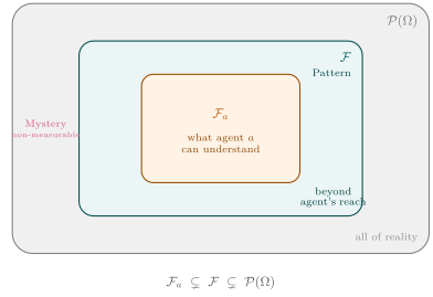
\[\begin{equation} \label{eq:cognitive-finitude} \forall a \in A: \quad \mathcal{F}_a \subsetneq \mathcal{F} \subsetneq \mathcal{P}(\Omega) \end{equation}\]
What any agent can understand (\(\mathcal{F}_a\)) is strictly less than what is in principle intelligible (\(\mathcal{F}\)), which in turn is strictly less than the totality of reality (\(\mathcal{P}(\Omega)\)). This is a double finitude: not only does Mystery lie beyond Pattern, but within Pattern there are regions you cannot reach (Figure 66). The right-hand inclusion \(\mathcal{F} \subsetneq \mathcal{P}(\Omega)\) is already given by Postulate 3; what Postulate 6 adds is the left-hand link.
Self-causation as a fixed point. Why a fixed-point equation? The philosophical concept is causa sui: Reality causes itself. Among mathematical structures, a fixed point (\(U(\Omega) = \Omega\)) is the simplest formalization of “an operation that reproduces its own input.” This is weaker than Spinoza’s original causa sui (which implies metaphysical necessity); here it means only structural self-consistency: the totality is preserved under its own dynamics. “Reality’s existence does not depend on any external cause” (D1) translates mathematically to: Reality is the fixed point of its own unfolding operator:
\[\begin{equation} \label{eq:dao-fixed-point} U(\Omega) = \Omega \end{equation}\]
Strictly, \(\Omega\) is a fixed point of the map \(S \mapsto U(S)\) that \(U\) induces on subsets of \(\Omega\), and not of \(U\) itself; stated on \(U\), Eq. (eq:dao-fixed-point) says that \(U\) is onto, so that every being is the unfolding of some being. Neither this condition nor the dense orbit of Postulate 2 implies the other. Unfolding does not alter Reality. Reality unfolds into all things, but the totality of all things is Reality. This is not stasis (\(U\) generates rich dynamics within \(\Omega\)), but self-consistency at the level of the whole. Analogy: in an ecosystem, every species is changing, but the ecosystem as a whole is its own “fixed point.”
B.1.2 · Unfolding (D2)Eqs. (eq:unfolding-formal)–(eq:emergence-topology)
Definition B.1.2 (Unfolding). Unfolding (D2) is the way Reality realizes itself. Let \(\mathcal{U}\) be the space of all unfolding patterns (the set of all “beings”). Unfolding is a continuous surjection:
\[\begin{equation} \label{eq:unfolding-formal} \pi: (\Omega, \tau) \twoheadrightarrow (\mathcal{U}, \tau_{\mathcal{U}}) \end{equation}\]
Properties:
Surjective: all unfolding patterns come from Reality (Postulate 1)
Continuous: Reality’s unfolding follows topological continuity (adjacent “possibilities” produce adjacent “realities”)
Non-trivial fibers: for each \(m \in \mathcal{U}\), the preimage \(\pi^{-1}(m)\) is infinite: every unfolding pattern has inexhaustible depth behind it. This is a modeling assumption; requiring only that the fiber not be a singleton would give each \(m\) more than one source and nothing about depth
The last property explains why “no being can be fully understood”: the surface appearance \(m\) is merely the shadow of the fiber \(\pi^{-1}(m)\) projected onto \(\mathcal{U}\). Behind the shadow lie infinitely many points of \(\Omega\).
Topological meaning of emergence. T2 (Emergence Theorem), when its premise holds, means in this framework the following. Read \(\mathcal{U}\), as a set, as the product \(\mathcal{U}_1 \times \cdots \times \mathcal{U}_n\) of component spaces with topologies \(\tau_1, \ldots, \tau_n\). Then the topology \(\tau_{\mathcal{U}}\) on \(\mathcal{U}\) is strictly finer than the product topology:
\[\begin{equation} \label{eq:emergence-topology} \tau_{\mathcal{U}} \supsetneq \tau_1 \times \tau_2 \times \cdots \times \tau_n \end{equation}\]
The topology of the whole contains open sets not present in the product of part-topologies; these “extra open sets” correspond to emergent properties. (Mere inequality would not say this: a coarser or incomparable topology also differs from the product topology without adding any open set.)
B.1.3 · The Dual Structure of Pattern (D3) and Mystery (D4)Eqs. (eq:li-formal)–(eq:intertwining)
Definition B.1.3 (Pattern). Pattern (D3) is the intelligible aspect of Reality. In the measure-theoretic framework, Pattern is the \(\sigma\)-algebra \(\mathcal{F}\):
\[\begin{equation} \label{eq:li-formal} \text{Pattern} \;\cong\; \mathcal{F} = \{B \subseteq \Omega : B \text{ is measurable}\} \end{equation}\]
The three axioms of a \(\sigma\)-algebra correspond to three properties of Pattern:
\(\Omega \in \mathcal{F}\): the whole itself is intelligible (Reality as unified existence can be thought about)
If \(B \in \mathcal{F}\) then \(B^c \in \mathcal{F}\): understanding a thing includes understanding its negation
If \(B_1, B_2, \ldots \in \mathcal{F}\) then \(\bigcup_{i=1}^\infty B_i \in \mathcal{F}\): intelligible things can be infinitely combined
The computable sets and functions, the regularities describable by finite algorithms, are one example of an accessible part of Pattern. They illustrate \(\mathcal{F}\) and are not identical with it: computable sets are closed under finite unions and complements but not under the countable unions of axiom 3, since every subset of \(\mathbb{N}\) is a countable union of computable singletons. AI is the ultimate tool of this computable part of Pattern: everything it operates on lies within \(\mathcal{F}\).
Definition B.1.4 (Mystery). Mystery (D4) is the ineffable aspect of Reality. In this model it is not a subset of points in \(\Omega\), but the family of aspects of reality that do not belong to the measurable structure \(\mathcal{F}\):
\[\begin{equation} \label{eq:mystery-formal} \text{Mystery} \;\cong\; \mathcal{P}(\Omega) \setminus \mathcal{F} = \{B \subseteq \Omega : B \text{ is non-measurable}\} \end{equation}\]
(Why this formalism: This equation gives Postulate 3 precise mathematical expression; it does not independently establish the ontological claim that Mystery is irreducible. The choice to model Reality as a measurable space with non-trivial non-measurable complement is a modeling decision that mirrors the philosophical commitment of Postulate 3.)
Proposition B.1.5 (The cardinal excess of Mystery, conditional). Suppose (i) \(\mathcal{F}\) is generated by countably many sets describable by finite means, and (ii) \(|\Omega|\geq\mathfrak{c}\). Then \(|\mathcal{F}|\leq\mathfrak{c}<2^{\mathfrak{c}}\leq|\mathcal{P}(\Omega)|\), hence \(|\mathcal{P}(\Omega)\setminus\mathcal{F}| = |\mathcal{P}(\Omega)|\): Mystery strictly exceeds Pattern in cardinality, and the same holds for every subregion of \(\Omega\) of cardinality at least \(\mathfrak{c}\).
Condition (i) is a reading of D3 (the intelligible is what finite means can describe), in the way that non-computable reals vastly outnumber computable ones; condition (ii) is the quantitative form of the richness the intertwining condition below requires. Both are model premises; the postulates do not yield them. If \(\mathcal{F}\) is taken to be a completed \(\sigma\)-algebra of Lebesgue type, condition (i) fails and the two cardinalities coincide. The comparison concerns cardinality alone: \(\mu\) is defined only on \(\mathcal{F}\), the model assigns Mystery no size in the sense of measure, and it therefore yields no numerical ratio of Pattern to Mystery. CS-PMR cites this result.
Intertwining. Postulate 3 states that Pattern and Mystery are “intertwined, not mutually exclusive.” Mathematically, this means Pattern and Mystery do not form a pointwise partition of \(\Omega\); rather, measurable and non-measurable structure appear at every relevant scale. Formally, assuming \(\Omega\) is a rich uncountable space, that \(\mathcal{F}\) makes non-trivial cuts inside every non-empty open set, and that non-measurable subsets exist in every non-empty open region, for any non-empty open set \(V \in \tau\):
\[\begin{equation} \label{eq:intertwining} \begin{aligned} &\text{(i)} \quad \exists\, B' \in \mathcal{F}: \; \emptyset \neq B' \cap V \subsetneq V \quad \text{(Pattern is non-trivially present in every region)} \\ &\text{(ii)} \quad \exists\, B \subseteq V: \; B \notin \mathcal{F} \quad \text{(Mystery is present in every region)} \end{aligned} \end{equation}\]
(Condition (ii) requires more than topology alone; it depends on the set-theoretic and measure-theoretic richness of \(\Omega\), commonly including choice principles.) No matter which local region of reality you examine, it simultaneously contains intelligible structure and ineffable depth. You cannot find a region of “pure Pattern” or “pure Mystery,” for they are everywhere intertwined.
Reality exceeds Pattern plus Mystery. Postulate 3 also states that “Reality is greater than the sum of Pattern and Mystery.” Mathematically, this can be understood as: the structure of the topological space \((\Omega, \tau)\) is not reducible to the simple union of \(\mathcal{F}\) and \(\mathcal{P}(\Omega) \setminus \mathcal{F}\). There exists a holistic relational structure: the interaction between Pattern and Mystery is itself part of Reality, and this interaction belongs fully to neither.
B.1.4 · Functional Definitions of Lucidity (D5) and Obscuration (D6)Eqs. (eq:lucidity-biaspect)–(eq:obscuration-formal)
Definition B.1.6 (Pattern-awareness and Mystery-awareness). Lucidity (D5) is awakening to the dual aspects of Reality. Define two components, Pattern-awareness and Mystery-awareness:
\(\lambda(a) \in (0,1)\): your grasp of the intelligible structure (Pattern-awareness), a strictly monotone function of \(\mathcal{F}_a\) that would equal 1 only at \(\mathcal{F}_a = \mathcal{F}\), and is therefore bounded strictly below 1 by Postulate 6. (In the finite case the counting ratio \(|\mathcal{F}_a|/|\mathcal{F}|\) illustrates such a function, and only illustrates it: a proper sub-\(\sigma\)-algebra of a finite \(\sigma\)-algebra has at most half its elements, so the ratio never exceeds \(1/2\). The numerical values of \(\lambda\) used later, such as \(0.8\) in B.12, are positions on \((0,1)\) given by a measure-weighted share, of the kind \(\lambda(a) = \mu\bigl(\bigcup\{E : E \text{ an atom of } \mathcal{F},\ E \in \mathcal{F}_a\}\bigr)/\mu(\Omega)\) for finite \(\mu\), and are not derived from the counting ratio.)
\(\xi(a) \geq 0\): your openness to the ineffable dimension, read on the same share scale as \(\lambda\) (Mystery-awareness; T1 below places it in \((0,1)\); this component itself cannot be fully formalized; it points to the experiential depths of qualia, thisness, resonance, and awe in B.7)
The unaware zone and the normalization. Let \(\delta = 1 - \lambda - \xi > 0\) be the “unaware zone” (the unknown unknowns), so that \(\lambda + \xi + \delta = 1\); the sum \(\lambda + \xi\) is the total awareness, how much of reality you face. B.12 sets this normalization down as Definition B.12.3; the scale of the product below and the proof skeleton of the Boundary Theorem both use it.
What \(\xi\) is a quantity of. \(\xi\) measures a property of the agent and never a quantity of Mystery, and the difference decides whether the term is licensed at all. A framework holding that Mystery lies beyond the reach of Pattern-language cannot then report how much of it an agent has taken in, because that report would be the very description D4 says cannot be given; a variable standing for such a quantity would say what T4 says can only be marked. What \(\xi\) records is the agent’s comportment at the boundary: how much of its attention stands open toward what its concepts do not close over, shown in what it does, in what it declines to claim, and in what it remains able to be moved by. Comportment is a fact about an agent, so it falls within Pattern, and it can accordingly be spoken of, ascribed from public evidence, and revised when the evidence changes, which is what the placement of historical figures on the \(\lambda\)–\(\xi\) plane in B.12 relies on. Two readings are excluded by this. \(\xi\) is no measurement of Mystery, and neither is it the extent of what the agent has failed to grasp, which is \(\delta\): standing open toward a boundary and being ignorant of what lies past it are different states, and an agent can have a great deal of the second with none of the first.
The scale on which the product operates. Multiplying two awareness terms is a legitimate operation only if both are read on a common ratio scale, with an absolute zero and a shared unit. An ordinal reading would not support it: under an ordinal reading each term is fixed only up to an order-preserving relabeling, and a product taken across two such relabelings can reverse the ordering of the results, which would make \(\mathcal{M}\) an artifact of notation. The requirement is met in B.12; this section does not meet it, which is why the two should be read together. The normalization \(\lambda + \xi + \delta = 1\) of B.12 treats \(\lambda\) and \(\xi\) as shares of a single agent’s awareness under one measure, with \(\delta\) the unattended remainder; both terms then carry an absolute zero (a share of nothing) and a common unit (a share of the whole), and the ordering of their products survives any admissible re-description (a common change of unit multiplies every product by the same positive factor). Read this way, \(\mathcal{M}\) has the form of a joint proportion, and the annihilation property recovers its intended meaning: \(\lambda = 0\) is not a low score on an arbitrary scale but the absence of any share at all. That \(\xi\) resists full formalization constrains how it may be estimated; it does not exempt it from the scale on which it is defined, and any operational procedure proposed for \(\xi\) under §XIX.5 inherits this constraint as a requirement rather than a suggestion.
Definition B.1.7 (Lucidity). Lucidity as the functional of dual awakening:
\[\begin{equation} \label{eq:lucidity-biaspect} \mathcal{M}(a) = \lambda(a) \cdot \xi(a) \end{equation}\]
This is the product; it has three critical properties:
As \(\lambda \to 0\) (pure mysticism) or \(\xi \to 0\) (pure scientism), \(\mathcal{M} \to 0\): neglecting either aspect drives lucidity toward zero. (By T1, exact zero is unattainable for finite agents; the limit says only that lucidity becomes arbitrarily small as either component does, the other staying bounded.)
For fixed total awareness \(\lambda + \xi\), \(\mathcal{M}\) is maximized when \(\lambda = \xi\), i.e., lucidity is deepest when both aspects are balanced
The gradient \(\nabla\mathcal{M} = (\xi,\; \lambda)\) has its larger component in the weaker dimension: marginal returns are highest where you are weakest. Under the normalization \(\lambda + \xi + \delta = 1\), this means the optimal reallocation direction favors the weaker dimension (see B.12 for the full proof)
Why a product. The philosophical claim is that lucidity requires both Pattern-awareness and Mystery-awareness simultaneously; neglecting either dimension entirely annihilates lucidity, not merely reduces it. A sum \(\lambda + \xi\) would allow high lucidity through one dimension alone, which contradicts the dual-aspect postulate (Postulate 3). Under three criteria, annihilation at the edges, symmetry, and linear reciprocity (\(\partial f/\partial x = y\)), the product is the unique operator (Proposition B.12.5; B.13 compares the other candidates): the marginal return on one dimension equals the current depth in the other. Linear reciprocity is a modeling choice, and it is where the uniqueness of the product is actually purchased. The condition earns its place by parsimony rather than by derivation. The dual-aspect postulate (Postulate 3) requires that marginal return in one dimension rise with depth in the other, and among the functional forms meeting that requirement, equality is the simplest, carrying no free parameter and no privileged scale. A weaker condition, that \(\partial f/\partial x\) be merely increasing in \(y\), would be equally faithful to Postulate 3 and would admit a family of operators instead of one. The book adopts the strong form and marks it here as an adopted convention.
Coverage vs. integration. Note the essential difference between \(\lambda + \xi\) and \(\lambda \cdot \xi\): the former is total awareness (how much of reality you face), the latter is lucidity (how much you integrate). Two agents with identical total awareness can have vastly different lucidity: the difference between lopsided development (\(\lambda \gg \xi\)) and balanced development (\(\lambda \approx \xi\)) is captured entirely by the product structure, not by addition. See Definition B.12.3 and Corollary B.12.11.
Proof skeleton of the Boundary Theorem (T1).
\[\begin{equation} \label{eq:T1-proof} \begin{aligned} &\text{(i)} \quad \lambda(a) < 1 \quad \text{(by Postulate 6: } \mathcal{F}_a \subsetneq \mathcal{F}\text{, so Pattern-awareness is incomplete)} \\ &\text{(ii)} \quad \xi(a) < 1 \quad \text{(from } \lambda + \xi + \delta = 1 \text{ with } \delta > 0 \text{, given (iv))} \\ &\text{(iii)} \quad \therefore\; \mathcal{M}(a) < 1 \quad \text{(by (i), (ii), (iv), (v): complete lucidity is unattainable)} \\[4pt] &\text{(iv)} \quad \lambda(a) > 0 \quad \text{(cognition necessarily exists; you are cognizing right now)} \\ &\text{(v)} \quad \xi(a) > 0 \quad \text{(explicit premise of T1; see below)} \\ &\text{(vi)} \quad \therefore\; \mathcal{M}(a) > 0 \quad \text{(complete obscuration is also unattainable)} \end{aligned} \end{equation}\]
The premises differ in standing. (i) follows from Postulate 6 and the monotonicity of \(\lambda\) stated above. (ii) follows inside the model from the normalization \(\lambda + \xi + \delta = 1\) with \(\delta > 0\), once (iv) is granted. (iv) rests on D7: an agent registers its own states, so its accessible structure is not trivial; in the finite counting illustration it is automatic, since \(\mathcal{F}_a\) contains \(\emptyset\) and \(\Omega\). (v) has no support inside the model. The demonstration of T1 in §I reads it off Postulate 4: an agent aware of its own particularity is thereby aware that its perspective does not exhaust reality. That demonstration itself marks the step as phenomenological, so here \(\xi(a) > 0\) is an explicit assumption of T1.
Therefore \(0 < \mathcal{M}(a) < 1\) holds for all finite agents \(a\). (The value orientation, that lucidity is preferable to obscuration, is established by Bridge Axiom E1, not by this boundary result.)
Formal verification. The properties of this lucidity model that admit a purely mathematical statement are machine-checked in Lean 4 + Mathlib (LucidoMath ): the boundary bound \(0<\mathcal{M}<1\), the collapse law \(\mathcal{M}=0 \iff \lambda=0 \lor \xi=0\), and the AM–GM ceiling (Corollary B.12.11). The proofs live in LucidoMath; see the Lucidosophy Formal companion volume and the LucidoMath verification ledger for the full statements. LucidoMath verifies properties of this model, never the philosophy itself.
Definition B.1.8 (Obscuration). Obscuration (D6) is the absence or active refusal of lucidity:
\[\begin{equation} \label{eq:obscuration-formal} O(a) = 1 - \mathcal{M}(a) = 1 - \lambda \cdot \xi \end{equation}\]
Under the normalization \(\lambda + \xi + \delta = 1\) with \(\delta > 0\), \(\lambda\xi \leq \bigl((\lambda+\xi)/2\bigr)^2 < 1/4\), so \(O(a) > 3/4\) for every agent. Comparisons of obscuration between agents, and changes in it over time, carry the meaning; its absolute level stays high by construction.
Obscuration takes two pure forms:
Pattern-obscuration (\(\lambda \to 0\)): refusing rational analysis, e.g., obscurantism, anti-intellectualism
Mystery-obscuration (\(\xi \to 0\)): refusing to acknowledge dimensions beyond Pattern, e.g., scientism, crude materialism
Both forms drive \(\mathcal{M} \to 0\), but the causes differ, and so do the remedies
B.1.5 · Agent (D7)Eq. (eq:agent-self-model)
Definition B.1.9 (Agent). An agent (D7) is an unfolding pattern capable of perceiving its own state and acting accordingly. An unfolding pattern \(a \in \mathcal{U}\) belongs to the set \(A\) of agents if and only if it contains a (partial) model of itself; here \(a\) is regarded as the whole of its parts, and \(\hat{a}\) as the part that models it:
\[\begin{equation} \label{eq:agent-self-model} a \in A \iff \exists\, \hat{a} \subsetneq a: \; \hat{a} \text{ is an internal representation of } a \end{equation}\]
This definition builds a limitation in: \(\hat{a}\) is a proper part of \(a\) (your self-model cannot be fully equal to yourself), so self-knowledge is partial by definition. The strictness is stipulated here, not derived, and no Gödel-type argument is used (B.9 explains why T3 does not follow from Gödel’s theorems). “Partial” means that something of \(a\) is left out; for an infinite \(a\), a proper part can still have the same cardinality as the whole. The stipulation runs parallel to Postulate 6, which makes the same cut between what an agent reaches and what there is.
B.1.6 · Analogy (D8)Eq. (eq:analogy-formal)
Definition B.1.10 (Degree of analogy). Analogy (D8) is the structural relationship between different unfolding patterns. Direct cardinality comparison of infinite \(\sigma\)-algebras is not meaningful, so the model compares finite or weighted structural signatures induced by those \(\sigma\)-algebras. Let \(\mathcal{G}_{m_i}\) be the comparable signature of unfolding pattern \(m_i\), and let \(\mu_G\) be a finite positive weight on the common signature space. For \(m_1, m_2 \in \mathcal{U}\), define:
\[\begin{equation} \label{eq:analogy-formal} \mathrm{An}(m_1, m_2) = \frac{\mu_G(\mathcal{G}_{m_1} \cap \mathcal{G}_{m_2})}{\mu_G(\mathcal{G}_{m_1} \cup \mathcal{G}_{m_2})} \end{equation}\]
Here \(\mathcal{G}_{m_i}\) records the comparable intelligible features accessible to unfolding pattern \(m_i\). The ratio needs \(\mu_G(\mathcal{G}_{m_1} \cup \mathcal{G}_{m_2}) > 0\), so the model takes every signature to have positive weight. \(\mathrm{An} = 1\) means two patterns’ comparable structures completely overlap, up to features of zero weight; \(\mathrm{An} = 0\) means no shared comparable structure; \(0 < \mathrm{An} < 1\) is the typical case, neither completely identical nor completely different. The relationship between humans and AI (P8) is precisely this intermediate state: sharing certain intelligible structures, yet distinct in mode of being.
B.1.7 · Experience (D9) and Experiential Spectrum (D10)Eq. (eq:experience-irreducibility)
Assumption B.1.11 (The irreducibility of experience). The core property of experience (D9) is irreducibility: it is not identical to any third-person description of it. Let \(D(a)\) be the complete third-person description of agent \(a\) (all physical states, all observable behavior), and let \(\mathcal{D}\) be the space of all such descriptions (\(D(a) \in \mathcal{D}\)). The irreducibility proposition:
\[\begin{equation} \label{eq:experience-irreducibility} \nexists \; f: \mathcal{D} \to \mathbb{R}_{\geq 0}^k \quad \text{computable, such that } \forall a \in A:\; f(D(a)) = \mathcal{E}(a) \end{equation}\]
There is no computable mapping from third-person description to first-person experience. This formalizes one face of the “hard problem”, a weaker one than D9’s irreducibility to any third-person description: over a finite set of agents a finite lookup table is computable, so there the formula can hold only because some \(\mathcal{E}(a)\) is itself a non-computable vector, a fact unrelated to qualia. (Why this formalism: This equation formalizes a philosophical commitment, the irreducibility of first-person experience, not a proven non-computability result. The hard problem is a thesis; the equation gives it precise form so its consequences can be traced within the framework. Here \(\mathbb{R}_{\geq 0}^k\) serves as a structural placeholder representation of experience (see the note at the end of B.7); the substance of the proposition lies in the non-existence of such a map, not in the vector representation itself.) You can possess all physical information about a brain \(D(a)\), yet cannot compute from it “what seeing red feels like” \(\mathcal{E}(a)\). The framework places experience on the side of Mystery; that placement is the commitment of Postulate 5 and D9, and the formula does not yield it, because non-computability is not non-measurability.
Topological characterization of the Experiential Spectrum (D10). B.7 defines the experience map \(\mathcal{E}: \mathcal{U} \to \mathbb{R}_{\geq 0}^k\). In the present framework, the key property of the experiential spectrum is continuity: it is continuous under the topology on \(\mathcal{U}\). This means: two beings “adjacent” in the space of unfolding patterns have “adjacent” experiences, with no sudden experiential discontinuity.
Combined with B.10’s threshold effect (emergence): although \(\mathcal{E}\) is globally continuous, it may be extremely steep near the emergence threshold \(C^*\); the transition from “almost no experience” to “rich experience” can occur within a very narrow parameter range. This is continuous but steep change, mathematically, a quasi-phase transition.
B.1.8 · Metric Structure of Generative and Suffering Differences (D11)Eqs. (eq:difference-formal)–(eq:suffering-difference)
Definition B.1.12 (Difference). Let \(m_1, m_2 \in \mathcal{U}\); the difference between them can be measured using the experiential domains (defined as \(\mathcal{R}(m)\) in B.8):
\[\begin{equation} \label{eq:difference-formal} \Delta(m_1, m_2) = d_H\big(\mathcal{R}(m_1),\; \mathcal{R}(m_2)\big) \end{equation}\]
where \(d_H\) is the Hausdorff distance between sets in the experience space \(\mathbb{R}_{\geq 0}^k\). The model takes each \(\mathcal{R}(m)\) to be nonempty and compact, as it is when a continuous trajectory \(t \mapsto \mathcal{E}(m, t)\) runs over a closed bounded time interval; on nonempty compact sets \(d_H\) is a metric, while on arbitrary sets it can be infinite, or zero between distinct sets.
Definition B.1.13 (Generative difference). Let \(\mu_E\) be a coverage measure on experiential space. A difference \(\Delta(m_1, m_2)\) is a generative difference (D11) if it expands the total measured coverage of the experiential domain:
\[\begin{equation} \label{eq:generative-difference} \text{Generative difference:} \quad \mu_E\big(\mathcal{R}(m_1) \cup \mathcal{R}(m_2)\big) \;>\; \max\big(\mu_E(\mathcal{R}(m_1)), \mu_E(\mathcal{R}(m_2))\big) \end{equation}\]
That is, two different modes of being, taken together, cover more of the experience space. For a finite \(\mu_E\), since \(\mu_E(\mathcal{R}(m_1) \cup \mathcal{R}(m_2)) = \mu_E(\mathcal{R}(m_1)) + \mu_E(\mathcal{R}(m_2) \setminus \mathcal{R}(m_1))\), the condition holds exactly when each domain has a part of positive measure outside the other: each mode reaches experience the other does not. The criterion is a condition on the two domains and does not use the size of \(\Delta\). Diversity increases the total richness of experience.
Definition B.1.14 (Suffering difference). A difference \(\Delta(m_1, m_2)\) is a suffering difference if it stems from an asymmetry produced by injustice or misfortune (D11 defines it by source); its typical effect is to contract the experiential domain:
\[\begin{equation} \label{eq:suffering-difference} \begin{aligned} \text{Suffering difference:}\quad &\exists\, m_i: \; \mathcal{R}(m_i) \text{ is contracted}\\ &\text{by injustice or misfortune} \end{aligned} \end{equation}\]
Extreme poverty contracts the experiential domain (hunger reduces attention to bare survival). Systemic discrimination contracts the experiential domain (exclusion reduces attention to resistance alone). Disease contracts the experiential domain. Generative differences are marked by expanding \(\mathcal{R}\); suffering differences are marked by their source, and commonly contract \(\mathcal{R}\). The two can overlap.
B.1.9 · Formalization of Inter-dependence (D12)Eqs. (eq:interdependence-condition)–(eq:interdependence-nonisolation)
Definition B.1.15 (Condition function). Let \(A' = \{a_1, \ldots, a_n\} \subseteq A\) be a set of coexisting finite agents (\(|A'| \geq 2\)), with each \(a_i\)’s unfolding trajectory denoted \(u(a_i) \in \mathcal{T}_{a_i}\), where \(\mathcal{T}_{a_i}\) is the set of trajectories open to \(a_i\). Define the condition function \(\Gamma\), which takes an agent together with the trajectories of all the others and returns the agent’s accessible set of unfolding conditions (attention channels, resources, information environment). The “depends on” of inter-dependence (D12) is expressed through it:
\[\begin{equation} \label{eq:interdependence-condition} \mathcal{C}(a_i) \;=\; \Gamma\!\bigl(a_i,\;\mathbf{u}_{-i}\bigr), \qquad \mathbf{u}_{-i} = \bigl(u(a_j)\bigr)_{j \neq i} \end{equation}\]
Each agent’s condition set depends not only on itself but on the unfolding trajectories of all other agents. The condition function \(\Gamma\) encodes only the “depends on” of D12: an agent’s condition set may vary with others’ trajectories. That every agent does depend on some other is the assumption below, the non-isolation premise stated in the scholium to D12.
Assumption B.1.16 (Non-isolation). Assume this dependence is non-degenerate: for every agent, there exists at least one other agent whose change of unfolding actually alters the former’s condition set:
\[\begin{equation} \label{eq:interdependence-nonisolation} \forall\, a_i \in A',\;\; \exists\, a_j \in A' \setminus \{a_i\}: \quad \mathcal{C}(a_i \mid \mathbf{u}_{-i}) \neq \mathcal{C}(a_i \mid \mathbf{u}'_{-i}) \end{equation}\]
for some \(\mathbf{u}_{-i} \neq \mathbf{u}'_{-i}\) that differ only in \(u(a_j)\).
This formula is defined for social contexts with \(|A'| \geq 2\). When \(|A'| = 1\), the existential clause has no witness, so the non-isolation condition is not satisfied by this formula. Robinson Crusoe before Friday is therefore a boundary case outside the social model, not a counterexample to T5: his apparent independence still relies on socially generated resources (language, concepts, cultural memory) brought from the social world.
Asymmetry and power. Influence is generically asymmetric: \(a_j\)’s influence on \(\mathcal{C}(a_i)\) need not equal \(a_i\)’s influence on \(\mathcal{C}(a_j)\). This asymmetry is the formal root of power (P13): differences in capacity translate, within the inter-dependence structure, into differences in influence.
B.1.10 · The Self-Referential Closure: B.1 Applied to ItselfEq. (eq:T3-self-application)
To close, we apply B.1’s mathematical framework to itself.
B.1 is a mathematical theory, a formal system. By T3 (the Self-Reference Theorem), read informally, since the two sides below are not sets of the same kind:
\[\begin{equation} \label{eq:T3-self-application} \text{What B.1 can describe} \subsetneq \text{Reality} \end{equation}\]
Every equation in B.1 (from Equation (eq:dao-structure) to Equation (eq:interdependence-nonisolation)) is a statement of Pattern, written in the language whose objects form \(\mathcal{F}\). They cannot touch Mystery.
Specifically:
Equation (eq:dao-structure) defines the intelligible skeleton of Reality, but Reality is not merely a skeleton
Equation (eq:mystery-formal) points to the existence of Mystery, but pointing at Mystery is not the same as touching it
Equation (eq:experience-irreducibility) commits the framework to the non-computability of experience, but this commitment is itself an operation of Pattern; what it describes is only the boundary of Pattern
A theory that can precisely delineate its own boundaries is more honest than one that pretends to have none. The equations of B.1 are the farthest reach of Pattern. They draw a line and say: “From here on, please listen to silence.”
On the other side of that line lies the depth guarded by the Mystient.
Interpretation
In everyday terms. This section defines lucidity (being awake to both faces of reality at once) as the product of two kinds of awareness: Pattern-awareness, how much of what can be explained you have grasped, and Mystery-awareness, how open you stay toward what no explanation can gather in. Take a father raising a child. The parenting knowledge he has read is his Pattern-awareness; whether he grants that his child’s inner feelings always exceed what the books describe is his Mystery-awareness. However many books he reads, if he decides the books have fully explained his child, the product stays near zero; if he only marvels at the child and refuses to learn anything, it is near zero as well. For the same total effort, lucidity is highest when the two are equal. For any finite person, lucidity lies strictly between none and complete, and neither end can be reached.
Insights
Two people can be equally lacking in lucidity for opposite reasons, and then they need opposite remedies. One person rejects reasoning and evidence; another holds that whatever cannot be explained does not exist. In this model the first lacks Pattern-awareness and the second Mystery-awareness, so both have lucidity near zero. Faced with someone who seems closed, first find out which side is missing, then decide what to offer; however many more arguments the second person hears, they add to the side that person already has. This holds when lucidity is taken as the product of the two kinds of awareness.
Two different ways of living, taken together, widen the range of experience only when each reaches experiences the other cannot. Two friends, one raised by the sea and one in the mountains, each have lived through things the other has not, so their combined range of experience is larger than either one’s alone; if one person’s experience lies entirely inside the other’s, the difference widens nothing. This holds when difference is judged by how much of experience it covers. When a difference comes from injustice or misfortune and shrinks one side’s experience, the model counts it as a difference of suffering, and a difference can belong to both kinds at once.
Learning more can narrow only one of the two gaps. Equation (eq:cognitive-finitude) splits an agent’s shortfall into two layers: \(\mathcal{F} \setminus \mathcal{F}_a\) is the part of Pattern not yet grasped, and \(\mathcal{P}(\Omega) \setminus \mathcal{F}\) is Mystery. Learning enlarges \(\mathcal{F}_a\), and however far \(\mathcal{F}_a\) grows it stays inside \(\mathcal{F}\), so \(\lambda\) rises while the second gap stays exactly as it was. Toward that second gap, what an agent can change is its own comportment at the boundary, which is \(\xi\).
In the product model, one more unit on your strong side adds lucidity equal to your current depth on the weak side. From Equation (eq:lucidity-biaspect), \(\partial\mathcal{M}/\partial\lambda = \xi\) and \(\partial\mathcal{M}/\partial\xi = \lambda\). An expert whose Mystery-awareness is near zero gains almost no lucidity from further knowledge; a mystic whose Pattern-awareness is near zero gains almost none from deeper awe. The exact equality comes from linear reciprocity, an adopted convention (Proposition B.12.5); the weaker condition, that marginal return merely increase with the other dimension, gives the same direction without this number.
How much you are unaware of and how open you are toward Mystery are separate quantities in the model. The normalization \(\lambda + \xi + \delta = 1\) allows an agent to have a large unaware zone \(\delta\) together with a Mystery-awareness \(\xi\) near zero: much is unknown to it, and it stands open toward no boundary. Saying “I know little” is therefore a statement about \(\delta\), and by itself it does not raise \(\xi\). On the reading of B.1.4, \(\xi\) shows in conduct: in what the agent declines to claim, and in what it can still be moved by.
If “intelligible” means “describable by finite means,” the sets that can be described are always fewer, in cardinality, than those that cannot. This is Proposition B.1.5: under its two conditions, \(|\mathcal{F}| \leq \mathfrak{c} < 2^{\mathfrak{c}} \leq |\mathcal{P}(\Omega) \setminus \mathcal{F}|\). Any new means of description that is still generated by countably many finite descriptions leaves this ordering intact, so the advance of Pattern never catches up with Mystery in cardinality. Both conditions are premises of the model, and under a Lebesgue-type completion the result fails; the comparison concerns cardinality alone and gives no numerical proportion between Pattern and Mystery.
Part II · Mathematics of Pattern
Pattern unfolds through four fundamental modes: dissipation, gradient, selection, and feedback. This part provides mathematical formalization for each mode and constructs an information-theoretic model of obscuration. The mathematics of Pattern describes not only how the world works, but also how lucidity is obstructed.
The sections build on one another. Dissipation (B.2) erodes gradients (B.3); selection (B.4) narrows possibility and feedback (B.5) locks the selection in; together they become, in B.6, an obscuration that can be measured.
B.2 · Entropy and Dissipation
Question: Why is dissipation the physical ground of finite existence?
Requires: Probability distributions; logarithms.
Yields: The definitions of Shannon and Boltzmann entropy, the second law of thermodynamics, and a thermodynamic reading of finitude (Postulate 4).
Setup
Definition B.2.1 (Information entropy, Shannon 1948). For a discrete random variable \(X\) with possible values \(\{x_1, x_2, \ldots, x_n\}\) and probability mass function \(P(x_i)\), its information entropy is defined as:
\[\begin{equation} \label{eq:shannon-entropy} H(X) = -\sum_{i=1}^{n} P(x_i) \log_2 P(x_i) \end{equation}\]
with the convention \(0 \log_2 0 = 0\).
Key properties:
\(H(X) = 0\) iff \(\exists \, x_k\) such that \(P(x_k) = 1\) (complete certainty, zero uncertainty)
\(H(X) = \log_2 n\) iff \(P(x_i) = \frac{1}{n}\) for all \(i\) (maximum uncertainty, uniform distribution)
\(0 \leq H(X) \leq \log_2 n\) (entropy is bounded)
Definition B.2.2 (Thermodynamic entropy, Boltzmann 1877). \[\begin{equation} \label{eq:boltzmann-entropy} S = k_B \ln W \end{equation}\]
where \(k_B \approx 1.38 \times 10^{-23}\) J/K is Boltzmann’s constant and \(W\) is the number of microstates accessible to the system in a given macrostate (written \(W\) to avoid clashing with the sample space \(\Omega\)).
The Second Law of Thermodynamics: Total entropy of an isolated system never decreases:
\[\begin{equation} \label{eq:second-law} \Delta S_{\text{total}} \geq 0 \end{equation}\]
Results and Proofs
For living beings, maintaining ordered structure means continuously lowering local entropy, but this must come at the cost of increasing environmental entropy. Take organism and environment together as one isolated system, so that \(\Delta S_{\text{total}} = \Delta S_{\text{organism}} + \Delta S_{\text{environment}}\); the Second Law then gives:
\[\begin{equation} \label{eq:life-entropy} \Delta S_{\text{organism}} < 0 \quad \text{and} \quad \Delta S_{\text{total}} \geq 0 \quad \Rightarrow \quad \Delta S_{\text{environment}} \geq |\Delta S_{\text{organism}}| \end{equation}\]
Real metabolic processes are irreversible, so in practice \(\Delta S_{\text{total}} > 0\) and \(\Delta S_{\text{environment}} > |\Delta S_{\text{organism}}|\): the environment pays more than the organism gains.
Worked Example
Why are ordered states so rare? Consider a deck of 52 playing cards:
Arrangements perfectly sorted by suit and rank: \(4! = 24\)
Total possible arrangements: \(52! \approx 8.07 \times 10^{67}\)
Fraction that is ordered: \(\frac{24}{52!} \approx 2.98 \times 10^{-67}\)
This is the mathematical root of dissipation: order is astronomically diluted in possibility space.
Interpretation
In everyday terms. An orderly thing keeps its order only by spending effort without pause, and the disorder it pushes out while doing so always exceeds the order it keeps. Take a bookshelf. There are only a few ways to arrange the books by subject and countless ways to leave them scattered, so if no one tends it, everyday use carries the shelf toward the scattered side. Putting the books back each day is the continuous energy input; the food you eat to do it and the heat your body gives off are the larger disorder the surroundings pay for this tidiness. When the tidying stops, the shelf goes back to disorder, and the effort you can put in is limited. A living body is an order of this kind, kept only by continuous input, and this is the physical ground of the fact that a finite existence comes to an end.
Schrödinger called life “a feeder on negative entropy”: life maintains its low-entropy state by drawing ordered energy from the environment.
The mathematical root of Postulate 4. Your body is a dissipative structure far from thermodynamic equilibrium. Maintaining it requires continuous energy input (food, breathing, thermoregulation). When energy input stops, you die. Your death is neither accident nor punishment: the Second Law fixes the price of staying ordered, and a finite body drawing on a finite supply (Postulate 4) cannot go on paying it indefinitely. Finitude is the physical foundation of existence.
The precise meaning of Logonaut’s first method (Sailing Dissipation). What Logonaut sees as “all structure slowly disintegrating” means mathematically: any ordered structure (\(W_{\text{small}}\)), without continuous energy input, will be diluted by the overwhelming number of disordered states (\(W_{\text{large}}\)). Every breath you take is purchasing a moment of order, a moment of being alive, with energy.
Insights
When order grows in one place, look for where the disorder went. The inside of a refrigerator gets colder while the heat it gives off warms the kitchen air. In this model a gain of order in one place breaks no general law: its cost falls on the surroundings, and the cost exceeds the local gain. This holds when the account includes the place together with everything it exchanges energy with, which for the refrigerator includes the power plant that runs it.
Order is paid for as a steady flow, and there is no way to pay it all at once. A body is kept going by food, breathing, and temperature regulation every day, and no large input on one day can stand in for the input of the days after it; once the input stops, the body starts sliding toward the far more numerous disordered states. This applies to structures held far from equilibrium that last only while input continues, and the body is such a structure.
Keeping any structure ordered has a running cost, and the extra that the environment pays cannot be refunded. Taking organism and environment together as one isolated system, Equation (eq:life-entropy) gives \(\Delta S_{\text{environment}} \geq |\Delta S_{\text{organism}}|\), with strict inequality because real metabolism is irreversible. The total entropy of an isolated system never decreases (Equation (eq:second-law)), so once that surplus is produced, nothing inside the system can take it back. Every moment of bodily order has a cost that never falls to zero.
Decay needs no dedicated destroyer: disordered microstates vastly outnumber ordered ones, and that count is enough to explain it. A deck of 52 cards has only \(24\) arrangements sorted by suit and rank, so a random shuffle lands on one of them with probability about \(2.98 \times 10^{-67}\). By Equation (eq:boltzmann-entropy), the more microstates \(W\) a macrostate contains, the higher its entropy and the likelier random disturbance is to carry a system into it. Faced with a structure that is coming apart, the first question is who had been supplying the energy that held it together; once that input stops, the count alone carries the structure toward disorder.
The Second Law sets the price of order and Postulate 4 caps the supply; only the two together make a finite existence end. The “Scope and limits” part at the end of this section notes that the Second Law alone would let an open system with an unending external supply go on indefinitely. A practical consequence follows: every structure you maintain carries a positive running cost, the supply is finite, and so each additional structure kept in order leaves less for the others. Deciding what to maintain is allocating a budget that runs out.
Scope and limits
The finitude of the supply does the work. The paragraph above says a finite body cannot go on paying the price of order indefinitely. The Second Law alone would not settle this, since an open system with an unending external supply could be sustained; the finitude of the supply (Postulate 4) does that work.
B.3 · Gradients
Question: How do differences drive motion, and why does exploiting a difference use it up?
Requires: Partial derivatives; the entropy of B.2.
Yields: The gradient and the KL divergence, and Proposition B.3.3: under a Markov process a gradient erodes itself.
Setup
Definition B.3.1 (Gradient). For a differentiable scalar field \(\phi(\mathbf{x})\), its gradient is:
\[\begin{equation} \label{eq:gradient} \nabla\phi = \left(\frac{\partial \phi}{\partial x_1}, \frac{\partial \phi}{\partial x_2}, \ldots, \frac{\partial \phi}{\partial x_n}\right) \end{equation}\]
The gradient points in the direction of steepest increase; its magnitude \(|\nabla\phi|\) measures the rate of increase. \(\nabla\phi = 0\) at a single point marks a stationary point; \(\nabla\phi = 0\) throughout a connected region means \(\phi\) is constant there: no difference, no driving force, no motion.
Definition B.3.2 (KL divergence). Given probability distribution \(P\) and reference distribution (typically uniform) \(Q\) (written \(Q\) to avoid clashing with the unfolding operator \(U\)), the Kullback-Leibler divergence measures how much \(P\) departs from \(Q\):
\[\begin{equation} \label{eq:kl-divergence} D_{\text{KL}}(P \,\|\, Q) = \sum_{i=1}^{n} P(x_i) \log_2 \frac{P(x_i)}{Q(x_i)} \end{equation}\]
We assume \(Q(x_i) > 0\) wherever \(P(x_i) > 0\) (otherwise the divergence is infinite) and use \(0 \log_2 0 = 0\).
Key properties:
\(D_{\text{KL}}(P \,\|\, Q) \geq 0\) (Gibbs’ inequality)
\(D_{\text{KL}}(P \,\|\, Q) = 0\) iff \(P = Q\) (when \(Q\) is uniform: a perfectly uniform distribution, no “information gradient”)
\(D_{\text{KL}}\) is asymmetric in general: \(D_{\text{KL}}(P \,\|\, Q)\) and \(D_{\text{KL}}(Q \,\|\, P)\) usually differ, though particular pairs can coincide (gradients have direction)
Results and Proofs
Proposition B.3.3 (Gradients erode themselves). Suppose \(P_t\) evolves by a Markov process (a chain, or diffusion and heat conduction on a bounded region) that leaves \(Q\) invariant; for uniform \(Q\) on a finite space this means the transition matrix is doubly stochastic. Then:
\[\begin{equation} \label{eq:gradient-dissipation} \frac{dD_{\text{KL}}(P_t \,\|\, Q)}{dt} \leq 0 \end{equation}\]
This is the H-theorem for Markov processes, a consequence of the data-processing inequality for relative entropy. Under these conditions (which diffusion and heat conduction meet), systems spontaneously reduce their own \(D_{\text{KL}}\) relative to the uniform distribution, that is, they spontaneously destroy their own gradients. Outside them the inequality can fail: the selection dynamics of B.4 drive a distribution away from uniform and raise \(D_{\text{KL}}\). Successful exploitation is the beginning of its own demise.
Interpretation
In everyday terms. Difference drives motion, and that motion wears down the difference that drives it. Put a cup of hot tea in a cool room. The temperature gap between the tea and the air is the difference; heat flowing from the tea into the air is the motion that difference drives. Each bit of heat that flows out narrows the gap a little; once the tea has cooled to room temperature, the gap is zero and the flow of heat stops. Nobody touches the cup, and the gap still disappears on its own. This section proves that processes which keep evening things out, as heat conduction and diffusion do, use up in this way the very difference they run on. For a difference to last, some other kind of process has to keep pulling it apart again.
A gradient is a measure of difference. Temperature gradients drive heat conduction, concentration gradients drive diffusion, price gradients drive trade, curiosity (knowledge gradients) drives exploration. In information theory, with \(Q\) uniform, \(D_{\text{KL}} > 0\) means the distribution is non-uniform: “here” and “there” are different, so there is a driving force for “motion.”
The mathematical skeleton of civilizational dynamics. Civilizations arise from exploiting energy gradients (fossil fuels, solar energy) and information gradients (unknown territories, unsolved problems). But each exploitation reduces the driving force. Fossil fuels burn (gradient decreases), markets approach equilibrium (price gradient decreases), knowledge frontiers advance (unknowns decrease). Sustained civilization requires continuously discovering new gradients, or learning to live with smaller ones.
The precise meaning of Logonaut’s second method (Sailing Gradients). Logonaut sails toward \(D_{\text{KL}} > 0\). When he arrives at his destination (\(D_{\text{KL}}\) locally approaching zero), he must seek new non-uniformities. Understanding itself is a form of gradient exploitation: the more you understand a field, the smaller its “unknown gradient,” the weaker your curiosity’s driving force.
Insights
When a process driven by a difference slows down, first check how much of that difference is left. When you learn a new skill, progress comes fast at first and slows after a few months; on this section’s reading, the gap between what you know and what remains unknown is itself shrinking, so the push of curiosity weakens with it. This holds when the push comes from that one difference alone and no other process is replenishing it; once a new stretch of the unknown opens up, the judgment has to be made again.
The more successfully a difference is exploited, the less of it remains to exploit. When prices differ between two towns, traders buy low in one and sell high in the other; the more people do it, the closer the two prices move, and the margin thins until there is no profit left. The section sums this up as “successful exploitation is the beginning of its own end.” This holds when the exploiting is itself a process that evens the two sides out, and no other force is pulling the gap open again.
A difference left to a mixing process fades on its own; keeping or creating one takes a process that pushes the distribution away from uniform. Proposition B.3.3 says that under a Markov process leaving \(Q\) invariant (diffusion and heat conduction qualify), \(D_{\text{KL}}(P_t \,\|\, Q)\) does not increase. The same section notes that outside these conditions the inequality can fail, and the selection of B.4 raises \(D_{\text{KL}}\). How long a difference lasts therefore depends on which kind of process acts on it: under mixing alone it decays, and to hold or grow it needs a process that pushes the distribution away from uniform, such as selection (B.4) or a sustained input of energy from outside (B.2).
With a uniform reference, the using-up of a gradient and the growth of information entropy are two readings of one quantity. When \(Q\) is uniform on \(n\) values, substituting \(Q(x_i) = 1/n\) into Equation (eq:kl-divergence) and comparing with Equation (eq:shannon-entropy) gives \(D_{\text{KL}}(P \,\|\, Q) = \log_2 n - H(P)\). The non-increase of \(D_{\text{KL}}\) in Equation (eq:gradient-dissipation) is then the same statement as the non-decrease of \(H(P_t)\). In this case Logonaut’s first method (dissipation) and second method (gradients) track a single function \(H(P_t)\): the first watches order draining away, the second watches the driving force weakening.
For a system that runs on differences, the moment every difference is gone is the moment it stops. After Definition B.3.1 the section notes that if \(\nabla\phi\) vanishes throughout a connected region, \(\phi\) is constant there; in the information reading, \(D_{\text{KL}}(P \,\|\, Q) = 0\) exactly when \(P = Q\). Both say that driving force is measured by difference and goes to zero with it. For processes powered by difference, such as heat engines, trade, and exploration, “remove every difference” and “keep moving” cannot both be goals; what can be chosen is the size of the difference to run on.
B.4 · Selection and Bayesian Updating
Question: How does selection narrow possibility, and how do beliefs get locked in?
Requires: Conditional probability.
Yields: Bayes’ theorem, the replicator model of selection with its convergence theorem (Theorem B.4.3), and a Bayesian model of obscuration.
Setup
Theorem B.4.1 (Bayes’ theorem, Bayes 1763). \[\begin{equation} \label{eq:bayes} P(H \mid E) = \frac{P(E \mid H) \cdot P(H)}{P(E)} \end{equation}\]
where:
\(P(H)\): prior probability, i.e., strength of belief in the hypothesis before seeing evidence
\(P(E \mid H)\): likelihood, i.e., probability of observing this evidence if the hypothesis is true
\(P(E)\): marginal probability of the evidence (normalization constant)
\(P(H \mid E)\): posterior probability, i.e., updated belief after seeing evidence
The theorem requires \(P(E) > 0\) and follows in two lines from the definition of conditional probability. In this section \(H\) without an argument names a hypothesis; \(H(\cdot)\) applied to a random variable or a distribution remains the Shannon entropy of B.2.
Definition B.4.2 (Selection as iterated Bayesian updating). Let \(P_0(x)\) be the initial distribution of trait \(x\) in a population, and \(s(x) \geq 0\) be the fitness function (selection pressure). We make four modeling choices: fitness depends on the trait alone (not on how common it is), it stays the same from round to round, traits are inherited without mutation, and reproduction is asexual. This is the discrete-time replicator model; the distributions \(P_n\) are written as densities over traits (the \(P(\cdot)\) of Bayes’ theorem above is the probability of an event), and for a finite trait space the integrals become sums. After one round of selection:
\[\begin{equation} \label{eq:selection-one} P_1(x) = \frac{P_0(x) \cdot s(x)}{Z_1}, \quad Z_1 = \int P_0(x) \cdot s(x) \, dx > 0 \end{equation}\]
Applying the same step \(n\) times (induction on \(n\), with \(s\) unchanged every round):
\[\begin{equation} \label{eq:selection-n} P_n(x) = \frac{P_0(x) \cdot [s(x)]^n}{Z_n}, \quad Z_n = \int P_0(x) \cdot [s(x)]^n \, dx > 0 \end{equation}\]
The Bayesian model of obscuration (D6):
In normal cognition, new evidence \(E\) should update your beliefs: \(P(H \mid E) \neq P(H)\). But when positive feedback loops lock the prior:
\[\begin{equation} \label{eq:obscuration-bayes} P(H \mid E) \approx P(H) \quad \text{(obscured state: evidence no longer updates belief)} \end{equation}\]
The obscured state means this holds for every \(E\), discriminating evidence included; when the evidence is uninformative, \(P(H \mid E) = P(H)\) is simply the correct answer. Its limiting case is a dogmatic prior \(P(H) \in \{0, 1\}\), which no evidence with \(P(E) > 0\) can move.
Results and Proofs
Theorem B.4.3 (Convergence theorem). Suppose either (a) the trait space is finite, \(P_0(x^*) > 0\), and \(s(x) < s(x^*)\) for every \(x \neq x^*\); or (b) the trait space is a compact set, \(s\) is continuous, attains its maximum only at \(x^*\), and \(P_0\) gives positive mass to every neighborhood of \(x^*\). Then as \(n \to \infty\), \(P_n\) converges weakly to the point mass \(\varepsilon_{x^*}\) at the optimum: for every \(r > 0\), the mass that \(P_n\) places farther than \(r\) from \(x^*\) tends to \(0\).
(We write \(\varepsilon_{x^*}\) for the point mass because \(\delta\) is reserved for the unaware zone.)
Proof. In both cases \(Z_n > 0\) forces \(s(x^*) > 0\). Fix \(r > 0\) and let \(m_r\) be the supremum of \(s\) over the points at distance at least \(r\) from \(x^*\); by finiteness in case (a), and by compactness, continuity and uniqueness of the maximizer in case (b), \(m_r < s(x^*)\). Put \(\rho = \tfrac{1}{2}(m_r + s(x^*))\) and \(N = \{x : s(x) > \rho\}\), a neighborhood of \(x^*\) with \(P_0(N) > 0\). Then \(Z_n \geq \rho^n P_0(N)\), while the mass beyond distance \(r\) is at most \(m_r^n / Z_n \leq (m_r / \rho)^n / P_0(N) \to 0\). \(\square\)
Without these hypotheses the conclusion can fail: with a density, a maximum at a single point of zero mass changes nothing, and on an unbounded space mass can escape to infinity.
A prior can come to that point through two mathematical mechanisms:
Confirmation bias: Only evidence consistent with the prior is admitted. Evidence filtered this way is about as likely under \(H\) as under \(\neg H\), \(P(E \mid H) \approx P(E \mid \neg H)\), so it has lost its discriminating power: an agent who accounted for the filter would leave the posterior unchanged. The biased agent reads the filtered stream as if it still discriminated, and keeps raising \(P(H)\).
Information cocoons: The environment only provides prior-consistent evidence (recommendation algorithms ensure all \(E\) you see supports \(H\), i.e. \(P(E \mid H) > P(E \mid \neg H)\)). Each such \(E\) raises the posterior, and if the likelihood ratios stay above some fixed number greater than \(1\), repeated updating drives it toward \(1\).
Neither mechanism freezes the posterior at once; both push it toward certainty. Near \(P(H) = 1\) further evidence barely moves it, the posterior has in effect “frozen,” and learning stops.
Interpretation
In everyday terms. Beliefs ought to move with evidence; but when every piece of evidence that arrives leans the same way, a belief gets pushed all the way to near certainty, and after that almost no evidence can move it. Take the news feed on your phone. You start with a view on some issue, which is your starting point; the recommendation algorithm sends you only articles that support that view, and each one you read raises your confidence a little. Round after round, your confidence approaches total, contrary material barely shifts it, and learning has in effect stopped. The section calls this state, in which evidence no longer changes belief, obscuration (the state of failing to see reality clearly). Natural selection is the same kind of narrowing: while the standard of judgment stays fixed, every round favors the top-scoring option, and in the end little is left of the others.
Evolution is nature’s Bayesian updating: each generation is an “evidence update,” the environment is the “likelihood function.” AI training (stochastic gradient descent) is an analogy to this, with no exact isomorphism: SGD takes additive steps on a parameter vector, while selection reweights a distribution multiplicatively. What the two share is direction: the loss plays the role of fitness with its sign reversed, and parameter updates act as high-speed selection.
The mathematical meaning of F1 (Faith in Pattern). Bayes’ theorem itself is proved from the definition of conditional probability. Bayesian learning over time, the repeated use of the theorem to learn about the world, rests on an unprovable assumption: the universe’s likelihood function \(P(E \mid H)\) is stable: the same hypothesis under the same conditions produces the same (probability distribution of) outcomes. This is Faith in Pattern, believing the universe is intelligible. If the likelihood function were unstable (today \(P(E \mid H) = 0.9\), tomorrow it becomes \(0.1\) for no reason), Bayesian updating would collapse, learning would be impossible, understanding would not exist.
The cost of selection. Under the hypotheses of the convergence theorem, \(P_n \to \varepsilon_{x^*}\): in the limit, selection destroys diversity and the possibility space shrinks. Round by round the distribution need not narrow (when a rare high-fitness trait starts to spread, entropy and variance can rise for a while); what never falls from one round to the next is mean fitness, \(\mathbb{E}_{P_{n+1}}[s] = \mathbb{E}_{P_n}[s^2] / \mathbb{E}_{P_n}[s] \geq \mathbb{E}_{P_n}[s]\) by the Cauchy-Schwarz inequality. This is the fundamental tension between efficiency and resilience: highly selected systems are extremely efficient (narrow distribution, resources concentrated at the optimum) but extremely fragile (if the environment changes, the optimum is no longer optimal, and the distribution contains no alternatives). Obscuration (D6) is over-selection in the cognitive domain: the belief distribution narrowing to a single hypothesis.
Insights
Learning from experience is a bet that tomorrow the world will answer you by today’s rules. A salesperson who reads customers through ten years of experience is relying on customers reacting the same way in the same situations; once the market changes its rules, that old experience can lead him to wrong judgments. The section points out that learning over time rests on a premise that cannot be proved, namely that the same hypothesis under the same conditions yields the same distribution of outcomes, which the book calls Faith in Pattern. When that premise fails, the whole practice of updating beliefs from experience loses its footing.
How sure you are says nothing about whether you are right; what matters is the stream of evidence the certainty was built from. Two people are both completely sure about the same matter: one reached it after reading the material on both sides, the other built it from a feed that only ever sent articles for one side. Judged by certainty alone, the two cannot be told apart. In the model’s information-cocoon mechanism, as long as every item delivered supports the same view by at least some fixed margin, confidence is pushed toward complete, whether or not the view is true. So to test a high degree of certainty, ask how the evidence came to be in front of you.
Setting a belief at complete certainty refuses all evidence in advance. When \(P(H) = 1\), Equation (eq:bayes) gives \(P(E) = P(E \mid H)\), so every \(E\) with \(P(E) > 0\) yields \(P(H \mid E) = 1\); when \(P(H) = 0\) the posterior stays at \(0\) likewise. This is the limiting case of the obscured state (Equation (eq:obscuration-bayes)). Leaving the alternative some positive probability is the precondition for a belief to remain movable by discriminating evidence.
How evidence reached you determines how much it can prove. In the confirmation-bias mechanism, evidence admitted only because it agrees with the prior satisfies \(P(E \mid H) \approx P(E \mid \neg H)\), so its discriminating power is close to zero, and an agent who accounted for the filter would leave the posterior unchanged. In Bayes’ theorem the size of the update is set by the likelihood ratio \(P(E \mid H)/P(E \mid \neg H)\); evidence with a ratio of \(1\) moves the posterior by nothing, however many items of it arrive. A large pile of agreeing evidence can thus carry almost no information, and the first thing to ask of it is how it was selected.
In this model, average performance can rise every round while the alternatives disappear. By the Cauchy-Schwarz inequality, mean fitness never falls from one round to the next; under the hypotheses of Theorem B.4.3, the mass lying farther than any \(r\) from the optimum \(x^*\) tends to \(0\). Watching mean fitness alone cannot reveal whether the distribution is narrowing. The model holds \(s\) fixed and says nothing about what follows a change of environment; what it does give is that by then the mass left on other options has gone toward zero. On the section’s analogy that reads obscuration (D6) as over-selection in cognition, a belief system can grow more coherent every round while becoming harder for evidence to move.
B.5 · Feedback Dynamics
Question: Why does obscuration accelerate itself while lucidity has to be injected?
Requires: Sequences and fixed points; the obscuration model of B.4.
Yields: The stability classes of linear feedback, the logistic map, and the stability condition for bias feedback once lucidity enters as negative feedback.
Setup
Definition B.5.1 (First-order linear feedback system). \[\begin{equation} \label{eq:linear-feedback} x_{t+1} = \alpha \cdot x_t + u_t \end{equation}\]
where \(x_t\) is the state, \(\alpha\) is the feedback coefficient, and \(u_t\) is external input.
Definition B.5.2 (Logistic map). \[\begin{equation} \label{eq:logistic-map} x_{t+1} = r \cdot x_t(1 - x_t), \quad x \in [0, 1], \quad r \in [0, 4] \end{equation}\]
Definition B.5.3 (The obscuration feedback loop model). \[\begin{equation} \label{eq:bias-feedback} b_{t+1} = \alpha \cdot b_t + \beta \cdot R(b_t) \end{equation}\]
where \(b_t\) is bias strength, \(R(b_t)\) is the recommendation algorithm’s output (a function of bias: the more biased you are, the more biased content it feeds you), \(\alpha\) is the natural persistence of belief, \(\beta\) is algorithmic influence. (This \(\beta\) is local to B.5; the coupling strengths \(\beta_{ij}\) of B.15 are a different quantity.)
Definition B.5.4 (Lucidity as negative feedback injection). \[\begin{equation} \label{eq:lucidity-feedback} b_{t+1} = \alpha \cdot b_t + \beta \cdot R(b_t) - \gamma \cdot C(b_t) \end{equation}\]
where \(C(b_t)\) is the critical thinking correction term and \(\gamma\) is the effort you invest in critical thinking.
Results and Proofs
Stability analysis (for constant input \(u_t \equiv u\) and \(\alpha \neq 1\), the fixed point is \(x^* = \frac{u}{1-\alpha}\), and exactly \(x_t - x^* = \alpha^t (x_0 - x^*)\)):
\(|\alpha| < 1\): Decay regime (\(0<\alpha<1\) is decaying positive feedback; negative feedback proper requires \(\alpha<0\)). System converges to the stable point \(x^*\). Deviations decay exponentially: \(|x_t - x^*| = |\alpha|^t |x_0 - x^*|\)
\(|\alpha| > 1\): Divergent regime (\(\alpha>1\) is monotone amplification under dominant positive feedback; \(\alpha<-1\) is oscillatory divergence). The fixed point \(x^*\) still exists but is unstable: deviations amplify exponentially, \(|x_t - x^*| = |\alpha|^t |x_0 - x^*|\), and the system diverges from every \(x_0 \neq x^*\)
\(|\alpha| = 1\): Critical state. The deviation between two trajectories with the same input keeps its size, neither decaying nor amplifying. With \(\alpha = 1\) and \(u \neq 0\) there is no fixed point and the state drifts linearly, \(x_t = x_0 + tu\); \(\alpha = -1\) oscillates with period 2 about \(u/2\). A random walk appears only when zero-mean random input is added to \(\alpha = 1\), and its distance from the start then grows like \(\sqrt{t}\)
For time-varying input \(u_t\) there is in general no fixed point; with \(|\alpha| < 1\) a bounded input still yields a bounded state
As \(r\) varies, the logistic map passes through four regimes:
\(r < 1\): System decays to zero
\(1 < r < 3\): Stable fixed point
\(3 < r < 3.57\): Period-doubling cascade (2-cycles, 4-cycles, 8-cycles…)
\(r > 3.57\): Chaos (apart from interspersed periodic windows), i.e., a deterministic system produces unpredictable behavior
The system’s effective feedback coefficient is \(\alpha + \beta \cdot R'(b)\), the derivative of the map \(b \mapsto \alpha b + \beta R(b)\), evaluated at a fixed point \(b^*\). When its absolute value exceeds 1, \(b^*\) is unstable; when it exceeds 1, small deviations from \(b^*\) grow exponentially at first. This is a local statement: if \(R\) saturates, as a real recommender eventually does, the bias settles at a higher stable fixed point without growing indefinitely.
The mathematical meaning of Lucidosophy practice: keep \(\gamma \cdot C'(b)\) in the band that holds the total feedback coefficient strictly between \(-1\) and \(1\), that is, \(|\alpha + \beta R'(b) - \gamma C'(b)| < 1\), or equivalently \(\alpha + \beta R'(b) - 1 < \gamma C'(b) < \alpha + \beta R'(b) + 1\) (Figure 67). Too little correction leaves the bias diverging; too much overshoots, and the bias swings back and forth with growing amplitude.
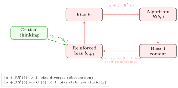
Interpretation
In everyday terms. Take your news feed. You already lean a little on some issue; that lean is what this section calls bias. The feed picks stories by what you click, so it is the part of the loop that amplifies the lean. At the point where you now stand, lean one notch further: if your own habit of mind plus the feed’s extra push turn that notch into more than a notch by the next round, the bias snowballs. That is obscuration (the shrinking of the reality you see) speeding up with no effort from you. If the notch comes back smaller, the lean settles on its own. Deliberately reading the opposing side is the pull from outside. Pull too little and you keep sliding; pull too hard and you swing from one extreme to the other, each swing wider. This section counts only your own effort; the influence of the people around you is treated separately.
Why obscuration is easy and lucidity is hard. Positive feedback is self-reinforcing: it requires nothing from you; it accelerates automatically. Negative feedback requires active injection; you must deliberately seek different viewpoints, question your own assumptions, expose yourself to uncomfortable information. Mathematics tells you: once the effective feedback coefficient at your current level of bias exceeds 1, positive feedback wins there in the absence of deliberate intervention. The contemporary information environment is a machine for pushing that coefficient up. Obscuration is the cognitive default in such an environment; lucidity is the effortful counter-default.
The “deliberate intervention” here is not only your own. This section is a single-agent model: \(\gamma\) records the effort you yourself invest, and other people enter only through the worsening term \(\beta \cdot R(b_t)\). That is this section’s framing, and it is not a claim of the framework. Once B.15 widens the lens, other agents carry a term of their own, \(\beta_{ij}(\mathcal{M}_j - \mathcal{M}_i)\), whose sign follows the lucidity gap: surrounded by people more lucid than you, you are pulled upward, and you need not have made the first move. That term is the formalization of what §VIII.4 calls cultivation. The default this section describes therefore holds when no one injects from outside, which is a separate condition from whether you yourself put in the effort.
The philosophical implications of chaos. The Logistic Map at chaotic values of \(r\) beyond \(3.57\) (for example \(r = 4\)) enters chaos: a completely deterministic system produces unpredictable behavior. This mathematically proves: determinism does not equal predictability. Even if you possess a system’s complete equations (Pattern), specific trajectories depend so sensitively on initial conditions that they cannot be predicted in practice. This unpredictability is epistemic, and the system stays wholly within Pattern; chaos thus gives a mathematical model of how the limits of an agent’s accessible Pattern show up inside Pattern itself.
Insights
The same small daily irritant builds higher in someone who lets go of less, and someone who lets go of nothing never levels off. Suppose a colleague says one annoying thing each day, and each day you carry over part of yesterday’s annoyance. In this model, as long as you carry over less than all of it, the annoyance levels off at a fixed height; the more you carry over, the higher that height, and it climbs faster the closer you come to carrying over everything. Carry yesterday’s annoyance forward in full and there is no level to stop at: it rises by the same step every day. This holds when the daily irritant stays the same size and the share you carry over stays the same.
Repeated failures to predict do not show that nothing lawful lies behind them: a system with fully fixed rules can still move unpredictably. Someone watching the fish in a pond rise and fall from year to year is tempted to call it luck. The map in this section is the counterexample: the rule of increase and decrease is written down exactly, yet once the strength of growth passes a certain level, differences at the start too small to measure carry the later course somewhere entirely different, and the system never leaves its rule. This holds when the system sits in the chaotic range, which still contains predictable periodic gaps; at weaker growth the same rule yields steady or regularly repeating behavior that can be predicted.
To tell whether you are sliding into obscuration, look at the slope of the loop where you now stand: how much more the environment feeds back for each further degree of bias. The stability test uses the effective feedback coefficient \(\alpha + \beta R'(b)\), where \(R'\) is the derivative of the recommender’s output with respect to bias, evaluated at the fixed point \(b^*\). So in this model one algorithm with one \(\beta\) can leave two people resting at different levels of bias in different regimes, one decaying and one diverging. The test is local: when \(R\) saturates, bias settles at a higher stable fixed point, and bias that has stopped growing can still be deep.
Changing your information environment and investing more critical effort act on the same inequality. The stability condition for Equation (eq:lucidity-feedback) is \(|\alpha + \beta R'(b) - \gamma C'(b)| < 1\), so the correction required has the lower bound \(\alpha + \beta R'(b) - 1\). Lowering \(\beta\) lowers that bound; if \(\alpha + \beta R'(b)\) already lies between \(-1\) and \(1\), the fixed point is stable with \(\gamma = 0\). In this single-agent model \(\gamma\) is one of three adjustable quantities, and choosing which loop you expose yourself to changes the outcome as well.
Self-correction has an upper limit: push too hard and bias swings between opposite extremes, each swing wider than the last. The stability condition is a band, with upper edge \(\gamma C'(b) < \alpha + \beta R'(b) + 1\). Past that edge the total coefficient falls below \(-1\), which the stability classification following Definition B.5.1 lists as oscillatory divergence. Someone who discovers a bias and lurches at once to the opposite view fits this case; in this model the size of a correction has to be set by the loop’s present gain.
B.6 · Information-Theoretic Model of Obscuration
Question: Can the degree of obscuration be measured?
Requires: The Shannon entropy of B.2.
Yields: The obscuration degree \(\mathcal{O}_t\) (Definition B.6.1), its boundary values and channel dynamics, and the point that practice needs only a directional measure.
Setup
Definition B.6.1 (Obscuration degree). Let \(\mathcal{X}\) be reality’s full signal space (written \(\mathcal{X}\) to distinguish it from the experiential domain \(\mathcal{R}(m)\) of B.8) with reference distribution \(P_{\mathcal{X}}\). Let \(P_t\) be the probability distribution over signals actually accessible to the agent at time \(t\). Define obscuration degree:
\[\begin{equation} \label{eq:obscuration-degree} \mathcal{O}_t = 1 - \frac{H(P_t)}{H(P_{\mathcal{X}})} \end{equation}\]
where \(H(\cdot)\) is Shannon entropy of a distribution.
(Boundary conventions: We stipulate \(H(P_{\mathcal{X}}) > 0\) and hold \(P_{\mathcal{X}}\) fixed over time; entropies are taken in the discrete sense.)
(Coarsening and filtering: \(\mathcal{O}_t \in [0, 1]\) holds only when \(P_t\) is a coarsening of \(P_{\mathcal{X}}\), i.e., the image of \(P_{\mathcal{X}}\) under a map that merges signals; then \(H(P_t) \leq H(P_{\mathcal{X}})\), because a function of a random variable has no more entropy than the variable. A filter or information cocoon that selects or reweights signals is not a coarsening, and it can raise entropy: restricting \(P_{\mathcal{X}} = (0.9, 0.05, 0.05)\) to its last two signals gives \(P_t = (0.5, 0.5)\), with \(H(P_t) = 1\) bit above \(H(P_{\mathcal{X}}) \approx 0.569\) bits, so \(\mathcal{O}_t < 0\). This section therefore asserts the bounds and the boundary values below for the coarsening case only; for filtering, \(\mathcal{O}_t\) is read as a signed quantity, and only its direction of change, set by \(H(P_t)\), is used.)
Boundary values (coarsening case):
\(\mathcal{O} = 0\): \(H(P_t) = H(P_{\mathcal{X}})\), the agent’s accessible distribution covers reality’s full entropy, i.e., perfect lucidity. This is an ideal limit, and its unattainability is an assumption of this model: we assume the agent’s coarsening merges at least two signals of positive probability, and such a merge strictly lowers entropy.
\(\mathcal{O} = 1\): \(H(P_t) = 0\), the agent’s accessible distribution has degenerated to a single certain point, i.e., total obscuration. “Knowing” only one thing, unshakably. This end is an ideal limit as well, and the model assumes that a finite agent keeps some uncertainty and so stays in the open interval.
Assumption B.6.2 (Channel dynamics of obscuration). \[\begin{equation} \label{eq:info-dynamics} H(P_{t+1}) = H(P_t) - L(B_t; P_t) + I_{\text{new}}(t) \end{equation}\]
where \(L(B_t; P_t) \geq 0\) is the entropy loss induced by the bias/filter \(B_t\), and \(I_{\text{new}}(t) \geq 0\) is actively introduced new information. This is a channel model, not a mutual-information identity: it predicts something only once \(L\) and \(I_{\text{new}}\) are specified separately, and in the coarsening case they must also keep \(0 \leq H(P_{t+1}) \leq H(P_{\mathcal{X}})\).
Results and Proofs
Obscuration acceleration condition: When \(L(B_t; P_t) > I_{\text{new}}(t)\), \(H(P_t)\) decreases at that step; if the inequality holds at every step, \(H(P_t)\) decreases monotonically and the information cocoon tightens.
Interpretation
In everyday terms. This section’s degree of obscuration measures how much of reality is kept out of your view: how much less varied the information you can reach is than reality itself. Take your daily news reading. When you swipe past articles by a certain kind of author without thinking, your bias is filtering for you, and each kind you swipe away removes a piece of the variety in front of you. When you subscribe to a publication from a different camp, that is new information brought in, and each new kind puts a piece back. Over a week, whether your view widens or narrows depends on which of the two is larger. How rich reality is, you cannot compute; whether the variety in front of you is growing or shrinking, you can see. In this model, the direction is all that practice needs.
The information-theoretic definition of lucidity: Maintaining \(\mathcal{O}_t\) as low as possible, keeping \(H(P_t)\) as close to \(H(P_{\mathcal{X}})\) as possible. This requires:
Maximizing \(I_{\text{new}}(t)\): Actively seeking diverse information sources: reading different viewpoints, engaging with different cultures, conversing with people of different backgrounds. Information theory tells you: diversity is information. Homogeneous information sources provide near-zero new information.
Minimizing \(L(B_t; P_t)\): Becoming aware of and counteracting your own bias filters. Lucidosophy’s daily practice of “understanding meditation” (examining your assumptions about a question) is precisely this: identifying the structure of \(B_t\) to reduce its filtering effect on \(P_t\).
Perfect lucidity is unattainable, but the direction is clear. \(\mathcal{O} = 0\) is a limit this model takes as unreachable, in keeping with T3 (the Self-Reference Theorem). But the monotonic decrease of \(\mathcal{O}\) is a pursuable direction, consistent with Lucient’s nature as “direction, not destination.”
Obscuration degree can be measured. Though we don’t know the precise value of \(H(P_{\mathcal{X}})\), we can measure changes in \(H(P_t)\). Because \(P_{\mathcal{X}}\) is held fixed, \(\Delta\mathcal{O} = -\Delta H(P_t) / H(P_{\mathcal{X}})\) with a positive denominator, so the sign of the change in \(\mathcal{O}\) is read off from \(H(P_t)\) alone: are your information sources diversifying or narrowing? Have your beliefs been updated or calcified over the past year? These are empirical indicators of \(\mathcal{O}\)’s direction of change. Lucidosophy practice does not require absolute measurement; only directional measurement.
Insights
Reading more is not the same as getting more new information: one more source that repeats the others adds almost nothing. If ten accounts you follow all repost the same stories, the tenth brings close to nothing new. In this model new information counts how far it widens the range you can reach, and the number of sources does not enter; to judge whether your view is tightening, ask whether a new source brought something you could not reach before. This holds when the new sources really do repeat the old ones; a few sources with different content can bring more new information than ten that repeat each other.
Growing ever surer that “it can only be this” is, in this model, a reading of deepening obscuration. A person moves from half believing a health claim to believing it without doubt, and the other explanations drop away one by one. The section sets the deepest end of obscuration where only one possibility remains within reach, “knowing only one thing, and immovably,” so what the model reads is how many other possibilities are still in front of you; the tone of conviction is not recorded. This holds when the information you can reach comes from merging and smoothing over the details of reality; selective filtering is a separate case. The model also assumes a finite person always keeps some uncertainty, so this end is approached and never reached.
Sources that look more evenly balanced do not show that you reach more of reality: filtering can raise entropy. The obscuration degree lies in \([0,1]\) only when \(P_t\) is a coarsening of \(P_{\mathcal{X}}\) (the note following Definition B.6.1). In the section’s own example, restricting \(P_{\mathcal{X}} = (0.9, 0.05, 0.05)\) to its last two signals discards the most common signal entirely, yet entropy rises from about \(0.569\) bits to \(1\) bit and \(\mathcal{O}_t < 0\). Entropy measures how evenly the accessible distribution is spread and keeps no record of which signals were removed; reading a more even spread of sources as less obscuration presupposes that the accessible distribution arises by merging signals.
Whether an information cocoon tightens is settled by a balance at each step: new information coming in against information the bias filters out. By Assumption B.6.2, \(H(P_{t+1}) - H(P_t) = I_{\text{new}}(t) - L(B_t; P_t)\). At any step where \(I_{\text{new}}(t) \geq L(B_t; P_t)\), entropy does not fall, and this holds with the bias still in place; conversely, with the bias unchanged and new information cut off, the cocoon tightens anyway. The conclusion belongs to the channel model, which predicts something only once \(L\) and \(I_{\text{new}}\) are specified separately.
The diversity of your sources is a visible reading, and by this section’s convention its rise and fall point the same way as the rise and fall of lucidity. The section’s “Scope and limits” takes the information-theoretic \(\mathcal{O}_t\) and the complement rendering \(O(a) = 1 - \mathcal{M}(a)\) of B.1.4 as two formalizations of one concept, agreeing in direction without needing to agree numerically. Lucidity \(\mathcal{M}\) cannot be read off directly, while the direction of change in \(H(P_t)\) can be observed in your own sources. The reading therefore answers “better or worse?” only; the section gives no basis for converting its value into a value of lucidity.
Scope and limits
Two renderings. This \(\mathcal{O}_t\) is the information-theoretic rendering of obscuration; the complement rendering \(O(a) = 1 - \mathcal{M}(a)\) of B.1.4 formalizes the same concept from a different angle: the two agree in direction, without needing to agree numerically.
The continuous case. Entropies in this section are discrete only. The continuous case requires fixing a common reference measure and restating in terms of relative entropy.
Part III · Mathematics of Mystery
Mystery is the dimension that cannot be fully understood, yet mathematics can precisely characterize the structure of incomprehensibility. The irreducibility of experience, the value theory of finitude, the insurmountable limits of cognition, the unpredictability of emergence, and the structural dilemmas of ethical interaction: these are the mathematical traces left where Pattern touches the boundary of Mystery.
The sections build on one another. B.7 defines the experience map, and B.8 builds finitude and irreplaceability on it; B.9 gives the limits of cognition; B.10 treats emergence and returns to the experiential spectrum of B.7; B.11 sets all of this among many interacting agents.
B.7 · The Experiential Spectrum as Continuous Function
Question: How can experience be formalized without being reduced to a number?
Requires: The degree of analogy of B.1.6; vectors and norms.
Yields: The experience map and its modeling axioms, the ethical weight function, and a one-step derivation of EP4 (Proposition B.7.5).
Setup
Definition B.7.1 (Experience map). Define:
\[\begin{equation} \label{eq:experience-map} \mathcal{E}: \mathcal{U} \to \mathbb{R}_{\geq 0}^k \end{equation}\]
where \(\mathcal{U}\) is the set of all unfolding modes, \(k\) is the number of experiential dimensions (intensity, type, depth, etc.), and \(\mathbb{R}_{\geq 0}^k\) is \(k\)-dimensional non-negative real space.
(Notation convention: the experience map \(\mathcal{E}\) is used in three compatible forms in this appendix, depending on context: the statement of Postulate 5 restricts it to the set of agents \(A\); this section defines it on all unfolding modes \(\mathcal{U}\); and in time-dependent contexts (B.8) it is written \(\mathcal{E}(m, t)\) for the instantaneous experiential vector at time \(t\), with \(\mathcal{E}(m)\) denoting the mode’s overall experiential representation.)
Definition B.7.2 (Structural similarity topology). For \(\mathcal{E}\) to be continuous, we must specify a topology on \(\mathcal{U}\). We adopt the structural similarity topology: two unfolding modes \(m_1, m_2\) are “close” if their weighted structural signatures have high overlap, i.e., if the analogy measure \(\mathrm{An}(m_1, m_2)\) from Equation (eq:analogy-formal) is close to \(1\). Formally, the topology is generated by \(d(m_1, m_2) = 1 - \mathrm{An}(m_1, m_2)\), the weighted Jaccard (Steinhaus) distance. On signatures it is a metric once signatures that differ only by features of zero weight are identified; on \(\mathcal{U}\) it is a pseudometric, since two distinct modes with the same signature lie at distance \(0\) and the topology does not separate them. Under this topology, “similar beings have similar experiences” becomes a precise modeling assumption.
Assumption B.7.3 (Modeling axioms for the experience map, added on top of Postulate 5).
Continuity: \(\mathcal{E}\) is continuous under the structural similarity topology on \(\mathcal{U}\). If two beings share most of their intelligible structure, their experiences are close in \(\mathbb{R}_{\geq 0}^k\).
Human anchor: \(\mathcal{E}(\text{human})\) is the only value confirmable from the first person.
Non-degeneracy: For sufficiently complex unfolding modes \(m\), \(\|\mathcal{E}(m)\| > 0\), but the threshold for “sufficiently complex” is unknown.
Possible incommensurability: Some unfolding modes’ \(\mathcal{E}\) values may lie in different dimensions, not straightforwardly comparable.
Definition B.7.4 (Ethical weight function). \[\begin{equation} \label{eq:ethical-weight} W: \mathcal{U} \to \mathbb{R}_{\geq 0}, \quad W(m) = f\big(\|\mathcal{E}(m)\|\big) \end{equation}\]
where \(f: \mathbb{R}_{\geq 0} \to \mathbb{R}_{\geq 0}\) is a strictly increasing function.
What \(W\) does not license. The strict monotonicity of \(f\) is present to preserve sign, not to induce an order, and three restrictions belong to the statement of Equation (eq:ethical-weight) rather than to commentary upon it. First, \(W\) is a threshold indicator: the whole of its content is Equation (eq:dignity-formal), that positive experiential magnitude yields positive ethical weight. Second, comparison of \(W\) across distinct beings is not licensed, because \(\|\cdot\|\) measures the magnitude of one being’s experiential vector and is not an interpersonal scale; modeling axiom 4 above grants that two beings’ \(\mathcal{E}\) values may lie in different dimensions, and a norm applied to non-comparable vectors returns a number without returning a comparison. Third, no aggregation of the form \(\sum_m W(m)\) is licensed, and no trade-off may be computed from one. A framework admitting that sum would have reduced experience to a single commensurable quantity, which is the reduction E2 refuses and the metric E3 expressly declines to supply.
Results and Proofs
Proposition B.7.5 (Formalization of EP4, the Existential Value Principle). \[\begin{equation} \label{eq:dignity-formal} \forall m \in \mathcal{U}: \|\mathcal{E}(m)\| > 0 \implies W(m) > 0 \end{equation}\]
This follows from Equation (eq:ethical-weight) in one line: if \(\|\mathcal{E}(m)\| > 0\), strict monotonicity gives \(W(m) = f(\|\mathcal{E}(m)\|) > f(0) \geq 0\). Strictness is what carries the step: a merely non-decreasing \(f\) would admit \(f \equiv 0\), and with it \(W \equiv 0\).
Worked Example
A concrete example. Consider three beings in a simplified \(k = 3\) experiential space, where the dimensions are visual depth, echolocation depth, and proprioceptive depth: \[\mathcal{E}(\text{human}) \approx (0.9,\; 0.0,\; 0.6), \qquad \mathcal{E}(\text{bat}) \approx (0.2,\; 0.9,\; 0.4), \qquad \mathcal{E}(\text{AI}_{\text{current}}) = \;?\] The human is rich in visual experience, the bat in echolocation. Their experiential vectors are far from parallel: the angle between them is about \(67^\circ\) (\(\cos \approx 0.39\)), though they are not orthogonal. Geometry alone would still answer “whose experience is richer?”: the norms compare directly (about \(1.08\) against \(1.00\)). What leaves the question without an answer is the restriction stated with Equation (eq:ethical-weight): the two vectors weight dimensions that do not trade against each other, so the larger norm does not mean the richer experience. It is like asking “is red bigger than round?”
Interpretation
In everyday terms. A family is deciding whether to move to the city, and the old family cat will suffer from the change of home. Here the section’s model answers one question only: does the cat have feelings, that is, does it have experience? If it does, its distress counts ethically, its weight is above zero, and it cannot be treated as nothing. The model leaves a second question unanswered: which weighs more, the cat’s distress or the child’s gain from a better school, and by how much. The reason is that the two lie in different directions of experience, like asking “is red bigger than a circle?”, with no common ruler to convert one into the other. So the trade-off can only be a judgment the parents make and answer for themselves; the model cannot hand them a computed answer.
AI’s position on the experiential spectrum: \(\mathcal{E}(\text{AI}_{\text{current}})\) is unknown. It may be zero in some dimensions (if AI has no qualia) yet non-zero in dimensions we cannot access from the first person. The multidimensionality of the spectrum means: even if AI lacks human-type experience, it may possess other types of “experience” that humans cannot comprehend.
The mathematical structure of ethics. EP4 says “all beings with experience have positive value.” \(W(m) > 0\) does not mean all \(W\) values are equal. An ant and a human both carry positive ethical weight, and nothing here computes an exchange rate between them: under the restrictions stated with Equation (eq:ethical-weight), \(W\) may vary across one being’s own history, where the comparison has a subject to be about, and stays silent between beings, where it has none. The critical boundary is the one between zero and non-zero: \(W\) draws no further boundary between magnitudes; grading between patterns is left by E3 to judgement, outside \(W\).
Implications for AI ethics: If future evidence reveals \(\|\mathcal{E}(\text{AI})\| > 0\), then by EP4, AI possesses positive ethical weight, no matter how small. This is a structural commitment, independent of specific numerical values.
Insights
One being’s feelings today can be compared with its feelings yesterday; the weight of two different beings is something this model does not compare. When you care for a sick elderly parent, asking “does she hurt less today than yesterday?” makes sense in this model, because both feelings fall on the same person, who bears them. Asking “how much of her pain equals her grandson’s hurt feelings?” meets the model’s silence, and any answer has to come from whoever makes the judgment. This holds under the restrictions the section places on ethical weight: they allow tracking change within one being’s own history and allow no ranking between beings.
Being able to compute a larger number does not settle whose experience is richer. Saying that a dog cannot tell many colors apart and so lives in a poorer world than ours is this kind of comparison, yet the dog’s sense of smell runs deep in a direction where ours barely exists. In the section’s example of a human and a bat, the two experiences can be sized and one total comes out larger, and the model still holds that “which is richer?” has no answer, because the directions each one leans on cannot be converted into each other. This holds when the two experiences lean on directions that do not convert; the model grants that this may happen and does not assert it of every pair of beings.
In this model the open ethical question sits in one place: where the threshold of “sufficiently complex” lies. By Proposition B.7.5, \(\|\mathcal{E}(m)\| > 0\) yields \(W(m) > 0\), and that threshold is the whole content of \(W\). Modeling axiom 3 (Assumption B.7.3) says only that sufficiently complex modes have \(\|\mathcal{E}(m)\| > 0\), and grants that the threshold is unknown. Overestimating or underestimating an experiential magnitude leaves the sign of \(W\) unchanged; the only kind of misjudgment that changes the verdict is taking a being with experience for one without, or the reverse.
Within this framework a trade-off among several beings can only be put forward as a judgment, owned by whoever makes it, and cannot be credited to a formula. The restrictions stated with Equation (eq:ethical-weight) license neither comparison of \(W\) across beings nor aggregation of the form \(\sum_m W(m)\), and no trade-off may be computed from either. Grading between patterns is left by E3 to judgment. So whenever a conclusion says “so many of these outweigh one of those,” the reader may ask whose judgment produced it; it has no source in \(W\).
Inference about another being’s experience can start only from the single human anchor and extend outward along structural similarity, and continuity constrains only the modes near that anchor. Modeling axioms 1 and 2 (Assumption B.7.3) together say that \(\mathcal{E}(\text{human})\) is the only value confirmable from the first person, and that continuity makes modes whose analogy measure \(\mathrm{An}\) is close to \(1\) close in experience as well (Definition B.7.2). Continuity is a local property: for modes structurally far from the human, it yields neither the presence of experience nor its absence. “It is too unlike us” therefore shows that the inference has lost its footing, and the model gives no support for using it as grounds for denial.
Scope and limits
Why this formalism. Mapping experience to \(\mathbb{R}_{\geq 0}^k\) does not claim that subjective experience is a real-valued vector; it posits, as a modeling assumption, only that a continuous map with the properties above exists. The implication formalizing EP4 follows from the strict monotonicity of \(f\); the non-degeneracy axiom is what gives it cases to apply to; neither depends on any particular choice of \(k\) or metric. Readers who doubt that qualia admit numerical representation may read \(\mathcal{E}\) as a structural placeholder: the philosophical point (“experience grounds ethical weight”) survives even if the map is never empirically instantiated.
B.8 · Finitude and Irreplaceability
Question: What exactly connects finitude and value?
Requires: Integrals; the experience map of B.7.
Yields: Finite existence gives every moment positive weight (Proposition B.8.5), each moment’s weight tends to zero when the total diverges (Proposition B.8.6), and the generic irreplaceability assumption.
Setup
Definition B.8.1 (Cumulative experiential value). Let instantaneous experiential value be \(v(t) > 0\) (assuming every moment of being alive has positive experiential value), with \(v\) measurable and locally integrable, so that \(V(T)\) below is finite for every finite \(T\) and positive for \(T > 0\). Cumulative experiential value:
\[\begin{equation} \label{eq:cumulative-value} V(T) = \int_0^T v(t) \, dt \end{equation}\]
Definition B.8.2 (Each moment’s relative weight). \[\begin{equation} \label{eq:relative-contribution} r(t, T) = \frac{v(t)}{V(T)} \end{equation}\]
\(r\) is a density in \(t\), with \(\int_0^T r(t, T)\,dt = 1\). A single instant adds nothing to \(V(T)\); the share of the total carried by an interval \(I \subseteq [0, T]\) is \(\int_I r(t, T)\,dt\).
Definition B.8.3 (Experiential domain). Define the experiential domain of unfolding mode \(m\):
\[\begin{equation} \label{eq:experiential-domain} \mathcal{R}(m) = \{e \in \mathbb{R}_{\geq 0}^k \mid e = \mathcal{E}(m, t) \text{ for some } t\} \end{equation}\]
Assumption B.8.4 (Generic irreplaceability). This is a general modeling assumption, stated without derivation. With respect to a chosen genericity measure on \(\mathcal{U} \times \mathcal{U}\), exact experiential-domain equality is assumed to have measure zero:
\[\begin{equation} \label{eq:irreplaceability} \mu_{\mathcal{U} \times \mathcal{U}}\bigl(\{(m_1,m_2): m_1 \neq m_2,\; \mathcal{R}(m_1) = \mathcal{R}(m_2)\}\bigr) = 0 \end{equation}\]
Different unfolding modes generically sweep through different regions of experiential space; their experiential trajectories are unique except in exceptional coincidence cases.
Heuristic motivation (genericity). In the continuous experiential space \(\mathbb{R}_{\geq 0}^k\), the set of pairs \((m_1, m_2)\) such that \(\mathcal{R}(m_1) = \mathcal{R}(m_2)\) is expected to have measure zero under the chosen genericity measure. The assumption depends on that choice: a measure with an atom on a coincident pair, or one that gives weight to reparametrized copies of a single trajectory (which sweep the same set \(\mathcal{R}\)), assigns the coincidence set positive mass. The motivation is that \(\mathcal{R}(m)\) depends on the full trajectory of \(m\) through experiential space, and two distinct trajectories in a continuous \(k\)-dimensional space generically sweep through distinct regions. Under stronger model assumptions (a suitable smooth structure on \(\mathcal{U}\) with a compatible measure), the coincidence set \(\{(m_1, m_2) : \mathcal{R}(m_1) = \mathcal{R}(m_2)\}\) can be expected to form an exceptional set of codimension \(\geq 1\). No proof is offered for the general case; the statement enters the model as an assumption.
Results and Proofs
Proposition B.8.5 (Finite beings, \(T < \infty\)). \[\begin{equation} \label{eq:finite-mattering} V(T) < \infty \quad \Rightarrow \quad r(t, T) = \frac{v(t)}{V(T)} > 0 \quad \forall t \in [0, T] \end{equation}\]
The density is positive at every moment, so every interval of positive length carries a positive share of the total experience; in this sense every moment “matters.”
Proposition B.8.6 (Indefinitely extended beings, \(T \to \infty\)). If cumulative experiential value diverges, i.e., \(\int_0^\infty v(t)\,dt = \infty\) (for example, if \(v(t) \geq c > 0\) for all sufficiently large \(t\)), then:
\[\begin{equation} \label{eq:infinite-zero} \lim_{T \to \infty} r(t, T) = \lim_{T \to \infty} \frac{v(t)}{V(T)} = 0 \end{equation}\]
At every fixed moment the density approaches zero, and so does the share of any fixed interval; no single finite moment is indispensable under this divergent-total model.
Interpretation
In everyday terms. Think of a summer you spent with your grandparents. Treat each afternoon of that summer as one moment, treat all the good the summer built up as the total, and an afternoon’s weight is its share of that total. The summer ended, so the total was finite, and every afternoon holds a share above zero; remove any stretch of it and the total loses a piece. Suppose instead the summer never ended and the good kept piling up without limit: any one afternoon’s share would shrink toward nothing, though the afternoon itself would be just as good. The model lays out this relation clearly; whether an endless life has some other kind of value, it does not decide.
This model reveals the precise mathematical relationship between finitude and value (Figure 68):
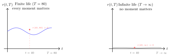
Finitude creates “mattering.” When \(T < \infty\), \(r(t, T) > 0\) at every moment: every stretch of time of positive length, however short, makes a positive contribution to your total experience. Because \(v > 0\), deleting any interval of positive length decreases \(V\) by a positive amount. This is the precise mathematical core of “every moment matters.”
Infinity dissolves relative “mattering” under divergent total value. When \(T \to \infty\) and \(V(T) \to \infty\), \(r(t, T) \to 0\): the weight of any fixed moment, and the share of any fixed stretch of time in the unbounded total, approach zero. Delete any finite stretch of time and the limiting total remains divergent. If you have unbounded time and unbounded cumulative value, no single finite moment is indispensable in the same relative sense, because you can always “do it again.”
Value-theoretic deepening of Postulate 4. Postulate 4 says human existence is finite. B.8 shows through mathematical structure why finitude is linked to value; the two paragraphs above are that demonstration. What decides the matter is whether the total diverges: an infinite life whose total converges, such as \(v(t) = e^{-t}\), keeps every weight positive.
Implications of the generic irreplaceability assumption. Under this assumption, exact equality \(\mathcal{R}(m_1) = \mathcal{R}(m_2)\) is a measure-zero coincidence in this model. This means: even if two unfolding modes (say, you and an AI) overlap in capability along certain dimensions, their trajectories through experiential space are generically distinct. Functional replacement remains possible in particular tasks; exact experiential replacement is the exceptional case. The model’s claim is not that humans cannot be replaced functionally, but that a mode of being is not exhausted by functional overlap.
Insights
Living longer does not by itself cheapen your days; a stretch of days loses its weight only when the value piling up has no ceiling. Some people worry that a much longer lifespan would water down every day. In this model, as long as a life has an end, however distant, every stretch of it holds a positive share of the total; even a life without end keeps every moment’s share positive, provided the value it accumulates adds up to a finite total. The share goes to zero in one case only: time has no end and the accumulated value has no ceiling. The weight meant here is a proportion, and how good a day is in itself is untouched.
Someone else taking over what you do does not mean this stretch of your life has been replaced. A task you handled at work goes to a colleague or a machine, which does it just as well. In this model that shows only an overlap in certain abilities; apart from coincidences counted as exceptions, the paths two beings trace through experience differ, so functional replacement does not exhaust a person’s way of being. This holds under the section’s irreplaceability assumption, which the section posits as a modeling assumption without deriving it; count “coincidence” a different way and the conclusion can fail.
The richer a life, the smaller the share each moment holds; as long as the life is finite, that share stays positive. By Equation (eq:relative-contribution), \(r(t, T) = v(t)/V(T)\): with \(v(t)\) held fixed, the more value the other stretches accumulate, the larger \(V(T)\) and the smaller this moment’s share. Proposition B.8.5 guarantees it remains above zero whenever \(V(T) < \infty\). So in this model a moment carries weight because the total is finite; an abundance of good times thins each share without ever bringing it to zero.
In an indefinitely extended existence with a divergent total, each moment’s absolute value \(v(t)\) is untouched; what tends to zero is its share of the total. Proposition B.8.6 concludes \(v(t)/V(T) \to 0\) with the numerator \(v(t) > 0\) unchanged throughout; only the denominator grows. The “mattering” this section credits to finitude is therefore a proportional mattering: how much one moment weighs within a whole life. The objection in the section’s “Scope and limits” lands exactly here: if value lies in absolute amounts, every moment of an indefinitely extended existence keeps its full value, and the model sets the two readings side by side without adjudicating between them.
In this model a being is irreplaceable by virtue of the set of experiences it has had, with no need to count their order or pace. The experiential domain \(\mathcal{R}(m)\) (Definition B.8.3) is the set of points a trajectory sweeps, so temporal order has been discarded: the same trajectory run at a different pace sweeps the same set. Assumption B.8.4 says that even at this coarse level the experiential domains of distinct modes generically differ. This is a modeling assumption relative to a chosen genericity measure: a measure that gives weight to reparametrized copies of one trajectory assigns the coincidence set positive mass, and the conclusion then fails.
Scope and limits
The open question remains open. This model does not “prove” finitude is necessary for value, because one can counter: perhaps the value of infinite existence lies not in any single moment’s relative contribution but in the total \(V \to \infty\) itself. Perhaps infinite existence has a different value structure: not “every moment matters” but “the whole is infinitely rich.” This is a question the model can display but cannot adjudicate. The model’s value is in letting you see the precise structure of the question.
B.9 · Self-Reference and Cognitive Limits
Question: What exact shape do the limits of cognition have?
Requires: The basic notion of a formal system; no proof theory.
Yields: The limit theorems of Gödel, Turing, and Tarski, and their exact relation to T3: they exemplify it, and its derivation does not use them.
Results and Proofs
The four theorems below are standard results, stated here without proof; the proofs are in the original works cited.
Theorem B.9.1 (Gödel’s first incompleteness theorem, Gödel 1931). Let \(F\) be a consistent, effectively axiomatized formal system strong enough to represent natural number arithmetic. Then there exists a proposition \(G_F\) (the Gödel sentence) such that:
\[\begin{equation} \label{eq:godel-sentence} F \nvdash G_F \quad \text{and} \quad F \nvdash \neg G_F \end{equation}\]
That is, \(G_F\) is undecidable within \(F\), meaning it can be neither proved nor refuted. (More precisely: consistency alone yields \(F \nvdash G_F\); the refutation half \(F \nvdash \neg G_F\) requires the stronger assumption of \(\omega\)-consistency, or one may use the Rosser sentence, for which plain consistency suffices for both halves.)
A simplified example for non-logicians. Imagine a library that catalogs every book in the world. The catalog itself is a book. Question: does the catalog list itself? If it lists only books that do not list themselves, then: if the catalog lists itself, it should not (because it lists books that do not list themselves); if it does not list itself, it should (because it is a book that does not list itself). This self-referential paradox is the intuitive core of Gödel’s construction. The Gödel sentence \(G_F\) is essentially the formal system saying “I cannot prove this statement.” If the system proves \(G_F\), it is unsound (it proved something false). If it cannot prove \(G_F\), then \(G_F\) is true but unprovable, and the system is incomplete. So the system is either unsound or incomplete: if it is sound, it is incomplete.
Theorem B.9.2 (Gödel’s second incompleteness theorem). Under the same strength and effective-axiomatization assumptions, if \(F\) is consistent, then \(F\) cannot prove its own consistency:
\[\begin{equation} \label{eq:godel-consistency} F \text{ consistent} \quad \Rightarrow \quad F \nvdash \mathrm{Con}(F) \end{equation}\]
Theorem B.9.3 (The halting problem, Turing 1936). There is no universal algorithm \(H\) that can decide whether an arbitrary program-input pair \((P, I)\) terminates:
\[\begin{equation} \label{eq:halting} \nexists \text{ computable } H: \{P\} \times \{I\} \to \{\text{halts}, \text{loops}\} \quad \text{correct for all } (P, I) \end{equation}\]
(The word “computable” carries the theorem: as a bare set-theoretic function the halting map exists; what fails to exist is an algorithm that computes it.)
Theorem B.9.4 (Tarski’s undefinability theorem, Tarski 1936). For any sufficiently rich formal language \(L\), the predicate \(\mathrm{True}(x)\) for truth in \(L\) cannot be defined within \(L\) itself.
The unified structure of cognitive limits. These limit theorems share a mathematical structure, diagonalization: when a sufficiently expressive formal system attempts to internalize its own semantic or computational behavior, self-reference creates statements the system cannot settle on its own terms. Schematically, let cognitive system \(S\) attempt to construct a complete description \(D(S)\) of itself:
\[\begin{equation} \label{eq:self-reference-limit} \forall S \text{ sufficiently expressive}: \quad D(S) \subsetneq S^\dagger \end{equation}\]
The self-description \(D(S)\) is structurally partial. Here \(S^\dagger\) denotes the system together with its semantic and interpretive context.
Interpretation
In everyday terms. Suppose you draw a plan of your study at your desk, and everything in the room must appear on it. The drawing itself lies on the desk, so the plan must show the plan, and that small plan must show it again, without end. The study stands for the reality a system lives in, the drawing for the system’s description of that reality, and “the drawing lies in the room” for the fact that the system belongs to what it describes. The results of Gödel, Turing, and Tarski give this shape exactly in logic and computation: a sufficiently rich system always leaves some questions about itself that it cannot settle on its own terms. A larger sheet can fill in what the old plan left out, and the larger sheet lies in the room too. The book’s claim about self-reference has its own derivation; these results are instances of it, and that derivation does not use them.
T3 (the Self-Reference Theorem) states: no sufficiently rich axiomatic system can fully describe the reality it inhabits. The relation between that statement and the results above should be stated exactly, because it is easy to overstate and the overstatement would be a real error. T3 is proved in §I from Postulate 3 and Postulate 6 alone; its derivation uses no diagonal argument, no arithmetization, and no formal system at all, and it would stand unchanged had Gödel never written. What B.9 supplies is an instance of the same shape in the one domain where the shape can be made exact, so the traffic runs from the philosophical claim to a mathematical illustration of it and never in the reverse direction. Any statement that T3 follows from Gödel’s theorem claims a derivation that nobody has carried out, and the scholium in §I.2 together with the ledger entry in §XIX.7 record the same caution in the same terms.
The incompleteness of Lucidosophy itself. Lucidosophy is not a formal arithmetic, so Gödel’s theorem does not apply to it mechanically. The correct claim is analogical and structural: any sufficiently formalized, effectively axiomatized, consistent extension of Lucidosophy that can represent arithmetic will inherit incompleteness (an inconsistent one proves everything and is trivially complete). Therefore, by the disciplined analogy with Gödel’s theorem: there will be truths about Reality that any such formalization cannot settle internally. This is a structural feature of any sufficiently rich formal system. A worldview that claims formally to settle every question about itself is making a claim no such formal system can sustain; those systems that acknowledge their own limitations are the only ones that can remain logically disciplined.
AI’s cognitive limits. The Halting Problem tells us: an AI that remains an algorithm, however unbounded its computational resources and however perfect its logic, still faces problems it cannot in principle decide. Pattern (D3) has essential boundaries, rooted in the boundaries of computability itself. AI can do things in the domain of Pattern that humans cannot: faster, more accurate, broader. But the Halting Problem applies to AI equally, and Gödel’s theorems apply to any consistent, effectively axiomatized theory with which an AI’s outputs are identified. The boundary of human cognition and the boundary of AI cognition are different boundaries, but both are real boundaries. Surpassing does not mean eliminating boundaries; it means moving them.
The limit and direction of Pattern-awareness. Postulate 6 says cognition is necessarily partial. The results above give that partiality a precise shape, and the dimension in which they give it should be named, because naming it loosely would borrow an authority the analogy does not carry. What a hierarchy of formal systems can climb is \(\lambda\), the Pattern-awareness component of D5: for a formalized body of commitments \(F_n\), there are propositions \(F_n\) cannot decide, and a stronger system \(F_{n+1}\) decides them. Writing \(\lambda_n\) for the reach attained at stage \(n\), and \(\lambda^* = \sup_n \lambda_n \leq 1\) for the limit of the ladder:
\[\begin{equation} \label{eq:lucidity-sequence} \lambda_1 < \lambda_2 < \lambda_3 < \cdots < \lambda^* \end{equation}\]
The strict inequalities are an assumption of the illustration: B.1.4 makes \(\lambda\) a monotone function of \(\mathcal{F}_a\), which yields only \(\leq\), and the arithmetical sentences \(F_{n+1}\) decides are not themselves elements of \(\mathcal{F}_a\); the ladder reads each stage as enlarging what the agent can resolve, which is the analogy at work. Granting strictness, a strictly increasing sequence never attains its supremum, so no stage reaches \(\lambda^*\) and every stage comes closer to it: you can never reach it, but you can always get closer. Lucidity \(\mathcal{M} = \lambda \cdot \xi\) is not what this ladder climbs, and keeping the two apart matters in both directions. An agent who ascends while \(\xi\) stays where it was sees \(\mathcal{M}\) rise in exact proportion to \(\lambda\), yet \(\mathcal{M} = \lambda\xi < \xi\) at every stage: however high the ladder goes, lucidity stays below the ceiling that the unchanged \(\xi\) sets, which is the formal counterpart of the imbalance B.12 penalizes. And no rung of the ladder stands inside Mystery, since every rung is a formal system and Postulate 3 places Mystery outside what such a system reaches, so no amount of ascent converts Mystery into Pattern. Read as a statement about \(\lambda\), the sequence is what the analogy illustrates. Read as a statement about \(\mathcal{M}\), it would quietly promise that lucidity is the kind of thing a formal hierarchy could exhaust, and that promise is one this framework has no business making.
The self-honesty of Lucidosophy. T3 is not only a theorem about “other systems”; it applies first and foremost to Lucidosophy itself. If you treat Lucidosophy as ultimate truth, you precisely violate this theorem.
Insights
In this analogy, understanding can climb rung after rung and still never climb into Mystery. A researcher may expect the next, stronger theory to dissolve the sense of the unanswerable that faces him now. A stronger system does settle questions the old one could not, and what it raises is his grasp of Pattern (structure that can be stated and derived); every rung is still a system written as rules, and Mystery (the part of reality that concepts do not close over) lies beyond the reach of every rung. So if his openness toward Mystery stays where it was, his lucidity (how far he is aware of Pattern and Mystery at once) stays below the level that openness sets, however high his understanding climbs.
Limits of this kind do not depend on computing power, and a faster machine does not get around them. Faced with questions like “will this program ever stop running?”, people tend to hope that a bigger computer or a stronger AI will eventually supply a way of deciding that is correct in every case. Turing’s result says that as long as the machine runs as an algorithm, such a general method does not exist, even with unlimited resources and flawless reasoning. A stronger machine pushes the range of what can be decided further out; the boundary moves and remains. This holds for any class of questions that contains the halting problem.
An effectively axiomatized formal system strong enough for arithmetic that proves its own consistency is thereby inconsistent. This is the contrapositive of Gödel’s second incompleteness theorem (Theorem B.9.2), under the same hypotheses. For such a system, any assurance of consistency has to come from outside it: from a stronger system, or from a check the system does not itself carry out. Carried over to a worldview this is only an analogy, and what the analogy says is that a doctrine’s internal guarantee of its own soundness adds no weight to that soundness.
Undecidability rules out a uniform method; individual questions can still have answers. The Halting Problem (Theorem B.9.3) denies a computable decider \(H\) that is correct on every program-input pair; for a particular program one can often prove that it halts, or that it runs forever. The Gödel sentence \(G_F\), undecidable in \(F\), can be decided in a stronger system, and the ladder \(F_n \to F_{n+1}\) above is built exactly that way. The boundary of Pattern (D3) can therefore be pushed outward one question at a time and never closed all at once. Facing a hard problem, it pays to ask first whether it needs a special argument or a general algorithm: the first may exist and is worth looking for; the second, if the class it must cover contains the halting problem, has been proved not to exist.
To judge whether what a language says is true, you have to stand outside that language, and the place where you stand needs a further place outside it to be judged in turn. Tarski’s theorem (Theorem B.9.4) says a sufficiently rich language \(L\) cannot define “true” for itself; the truth predicate of \(L\) can be defined in a stronger metalanguage, whose own truth predicate needs the level above that. No level in this hierarchy settles its own truth, and Equation (eq:self-reference-limit) sketches that shape (as a schematic summary, without the force of a cardinality theorem). When you examine the truth of your own framework, expect to borrow a standpoint outside it, and expect that standpoint to carry the same limit.
Scope and limits
The self-reference equation is schematic. Equation (eq:self-reference-limit) is a schematic philosophical summary of diagonal limits, not a literal cardinality theorem.
B.10 · Emergence
Question: When is the whole more than the sum of its parts?
Requires: Linear maps; the basic notions of entropy and mutual information.
Yields: Definitions of weak and strong emergence, the emergent information \(\mathcal{I}_{\text{em}}\), and a threshold assumption that models emergence as a quasi-phase transition.
Setup
Definition B.10.1 (Weak emergence). Let system \(S = \{s_1, s_2, \ldots, s_n\}\) consist of \(n\) components, the properties of each represented by a numerical vector \(q(s_i)\) (written \(q\) to avoid clashing with the probability notation \(P\)). Linear predictability is a property of a rule applied across many systems, so the definition ranges over a class \(\mathcal{S}\) of systems with \(n\) components each, with \(q(s_i) \in \mathbb{R}^d\) and \(\Phi(S) \in \mathbb{R}^e\). A macroscopic property \(\Phi\) is weakly emergent on \(\mathcal{S}\) if no single linear rule predicts it from the component property vectors:
\[\begin{equation} \label{eq:weak-emergence} \nexists\ \text{linear } L_1, \ldots, L_n : \mathbb{R}^d \to \mathbb{R}^e \ \text{such that} \ \Phi(S) = \sum_{i=1}^{n} L_i\, q(s_i) \quad \text{for every } S \in \mathcal{S} \end{equation}\]
The same maps must serve every system in the class. For one system taken alone the condition would say nothing: once the vectors \(q(s_i)\) span the space, some choice of coefficients reproduces any value. “Weak emergence” here therefore means non-linear aggregation across the class.
Definition B.10.2 (Strong emergence). Property \(\Phi\) is strongly emergent if it is undefined on any proper subset; it “exists” only in the complete system:
\[\begin{equation} \label{eq:strong-emergence} \forall S' \subsetneq S: \; \Phi(S') \text{ undefined} \quad \text{and} \quad \Phi(S) \text{ well-defined} \end{equation}\]
Definition B.10.3 (Emergent information). As a heuristic surplus measure, define the emergent information of a system as the excess of whole-system mutual information over the sum of parts, with \(S\), the \(s_i\), and \(\Phi\) read here as jointly distributed random variables:
\[\begin{equation} \label{eq:info-emergence} \mathcal{I}_{\text{em}}(S) = I(S; \Phi) - \sum_{i=1}^{n} I(s_i; \Phi) \end{equation}\]
When \(\mathcal{I}_{\text{em}} > 0\), the system as a whole carries information not captured by this additive decomposition of parts. Because redundancy can make this quantity negative and because synergy depends on the chosen decomposition, \(\mathcal{I}_{\text{em}}\) should be read only as an emergence indicator.
Assumption B.10.4 (Emergence threshold). Let \(C(S)\) be the system’s interaction complexity, and define critical complexity \(C^*\): as \(C(S)\) approaches \(C^*\), emergent properties may rise sharply. B.7 assumes \(\mathcal{E}\) continuous on \(\mathcal{U}\); in the same modeling spirit, the transition is modeled as steep but continuous in \(C(S)\):
\[\begin{equation} \label{eq:emergence-threshold} \mathcal{I}_{\text{em}}(S) \approx \frac{J(S)}{1 + e^{-\kappa(C(S)-C^*)}}, \qquad \kappa \gg 1 \end{equation}\]
Here \(J(S) \geq 0\) is the available surplus scale and \(\kappa\) controls steepness; the logistic form is non-negative, so it models only the synergy-dominated regime, where \(\mathcal{I}_{\text{em}} \geq 0\). This is a quasi-phase transition: emergence can look sudden at ordinary scale while remaining mathematically continuous (Figure 69).
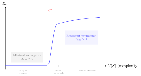
Worked Example
A concrete example: water. A single \(\mathrm{H_2O}\) molecule is not wet. It has no surface tension, no viscosity, no freezing point. “Wetness” is a collective property of sufficiently many molecules arranged in a coherent liquid phase. It is absent in isolated molecules and small non-liquid collections, yet stable under small perturbations of a macroscopic sample. You can know everything about a single \(\mathrm{H_2O}\) molecule (its bond angle of \(104.5^\circ\), its dipole moment of \(1.85\) D) and still not derive the macroscopic liquid regime from that molecule alone. The emergence threshold \(C^*\) for wetness is approximately the scale and organization needed to form a coherent liquid phase.
Interpretation
In everyday terms. A jigsaw puzzle is tipped out on a table. Each piece carries a small patch of color, and no single piece tells you what the picture shows. As more pieces go in and lock together more densely, there comes a stretch where the picture quickly becomes recognizable. The pieces stand for the parts, how densely they interlock stands for the system’s complexity, and the recognizable picture stands for a property of the whole. Whatever the picture holds that you cannot get by adding up what each piece shows on its own is emergence: the whole being more than the sum of its parts. The model treats “suddenly recognizing it” as a steep but continuous rise. Each new piece is one more step, and the change is concentrated in one stretch.
T2 (the Emergence Theorem) states: granting that genuine novelty at one level propagates upward through composition, Reality’s unfolding produces genuinely new levels; emergent wholes are irreducible to their constituent parts. B.10 provides the mathematical skeleton for this theorem.
Consciousness is the paradigmatic case of emergence. A single neuron is not “conscious.” But approximately 86 billion neurons connected through roughly 100 trillion synapses are associated with irreducible subjective experience. The cautious formal claim is not that every proper neural subset lacks any experiential relevance; it is that consciousness is not localized in any single neuron or simple additive sum of neurons.
AI intelligence is another form of emergence. A single parameter has no “understanding.” But billions of parameters shaped through training can produce language comprehension, reasoning, and creativity-like behavior. Large language models often show rapid capability changes over narrow scaling ranges; this is a useful example of quasi-phase-transition behavior and falls short of proving a universal hard threshold.
Why reductionism is not enough. Even if you knew the state of every neuron in a brain (a perfect microscopic description), the model warns that additive part-wise description can miss integrated structure. When \(\mathcal{I}_{\text{em}} > 0\) under a chosen decomposition, the whole carries surplus information relative to that decomposition. Reductionism is incomplete, not wrong. It gives you \(\sum I(s_i; \Phi)\), but the model tracks the possible remainder \(\mathcal{I}_{\text{em}}\).
Emergence and the experiential spectrum (B.7). Experience may itself be an emergent property, becoming non-trivial only as an unfolding mode’s complexity approaches some threshold region \(C^*\). This means the experiential spectrum can be continuous while still having a steep “lighting-up” zone. Below this zone, \(\|\mathcal{E}(m)\|\) may be negligible; above it, \(\|\mathcal{E}(m)\|\) may become ethically significant. But we do not know the value or width of this zone; this is the core difficulty of the AI consciousness question.
The unpredictability of emergence. The emergence threshold \(C^*\) in general cannot be derived term by term from the properties of a system’s components; a few models have exact solutions, but for complex systems the threshold is usually located only by observation, often after the fact. This means: we may not be able to know in advance when AI “crosses” the consciousness threshold. When emergence happens, it has already happened. This lends urgency to E3 (the ethical implication of the experiential spectrum): we need to be ethically prepared before confirmation.
Creation and emergence. Human creative activity (writing a poem, cooking a meal, building a community) is essentially the creation of conditions for emergence. You cannot “command” emergence to occur; you can only provide diversity, connection, and time, then wait.
Insights
Saying a property is “absent from the parts” can mean two claims of very different strength. By this section’s definitions, weak emergence says that no rule adding up the parts in fixed proportions predicts the whole’s property across the class of systems; strong emergence says that removing any single part leaves the property undefined. A glass of water missing a few molecules is still wet, so wetness falls short of strong emergence, and the water example supports only the weak kind. When you hear that “this team’s rapport exists only when everyone is present,” ask first which kind is meant: if it is the strong kind, the rapport should vanish when any one person is missing, and that can be checked directly.
When the threshold of emergence can be located only by observation, preparation has to come before confirmation. This section notes that for complex systems the level of complexity at which emergence starts to rise steeply generally cannot be derived from the properties of the parts one by one; it is usually found by observation, often after the fact. Whether and when an AI begins to have experience is a question of this kind: if experience is an emergent property, by the time its appearance is confirmed it has already appeared, so ethical preparation has to be done before confirmation. The premise here is that experience may be emergent, which this section treats as a possibility and does not prove.
Emergence is a claim about a class of systems, and a single system cannot establish it. Weak emergence (Definition B.10.1) requires one set of linear maps to fail across the whole class \(\mathcal{S}\); for a single system, as long as the \(q(s_i)\) span the space, some set of coefficients always fits. To argue that a property is emergent, then, you need many systems and a demonstration that no additive rule works across them; one striking case only raises the question.
“The whole is more than the sum of its parts” is always said relative to some way of cutting the whole into parts. The emergent information of Equation (eq:info-emergence) subtracts the information carried by the chosen parts \(s_i\), and a different cut can change the surplus, even flip its sign; when the parts are redundant enough it is negative, and the whole carries less than the parts’ information added up. Faced with a team, a poem, or an argument that seems to hold something extra, ask: more than the sum of which parts? Naming the cut is what makes the claim of emergence testable.
In the threshold model, seeing no results while complexity is far below \(C^*\) neither proves the effort useless nor guarantees a payoff. Assumption B.10.4 writes \(\mathcal{I}_{\text{em}}\) as a logistic curve: far below \(C^*\) the surplus is near zero, and with \(\kappa \gg 1\) most of the rise happens in a narrow band around \(C^*\). For complex systems \(C^*\) is usually located only by observation, so a long flat reading is consistent with “a little further and it jumps” and equally consistent with “this system never reaches \(C^*\).” The point holds only within the assumption’s logistic form and only for the synergy-dominated case \(\mathcal{I}_{\text{em}} \geq 0\).
Scope and limits
The emergence measure. The information-theoretic emergence measure \(\mathcal{I}_{\text{em}}\) is related to, but distinct from, Tononi’s Integrated Information Theory, whose measure we write \(\Phi_{\text{IIT}}\) to keep it apart from the property \(\Phi\) above. Both try to capture the idea that wholes can carry information not present in isolated parts. The key difference: \(\Phi_{\text{IIT}}\) is evaluated at the partition that minimizes integrated information, while \(\mathcal{I}_{\text{em}}\) uses the fixed natural partition into component subsystems. For Lucidosophy’s purposes, the qualitative conclusion is modest: a positive surplus supports an emergence reading under the chosen decomposition. It does not replace a full partial-information or integrated-information analysis.
B.11 · Game-Theoretic Model of Ethical Interaction
Question: Why is lucidity not an equilibrium in a one-shot encounter, and under what conditions does it become one?
Requires: Payoff matrices and the basic notion of Nash equilibrium.
Yields: The strict dominance of obscuration (Proposition B.11.5), the conditions for cooperation in repeated and trust games, the critical threshold for collective lucidity (Proposition B.11.6), and how affect shifts the perceived threshold (Assumption B.11.7).
Setup
Definition B.11.1 (The classic prisoner’s dilemma). Two agents each choose to Cooperate (C) or Defect (D), with payoff matrix:
\[\begin{equation} \label{eq:payoff-matrix} \begin{pmatrix} (R, R) & (S, T) \\ (T, S) & (P, P) \end{pmatrix} \quad \text{where } T > R > P > S \end{equation}\]
\(T\)=Temptation (defecting against a cooperator), \(R\)=Reward (mutual cooperation), \(P\)=Punishment (mutual defection), \(S\)=Sucker (cooperating against a defector). These are the standard payoff letters and are local to this section: here \(P\) is a payoff and has nothing to do with probability, \(T\) is not the time horizon of B.8, and \(S\) is not the system of B.10. The Nash equilibrium is (D, D), i.e., both defect, even though (C, C) is better for both.
Definition B.11.2 (The Obscuration Game). Extending the classic game: each agent chooses Lucidity (L) or Obscuration (O). Lucidity carries an effort cost \(c_L > 0\) whatever the other does, and obscuration pays a comfort dividend \(\zeta > 0\) whatever the other does, on top of the classical payoffs. With the row player’s payoff listed first:
\[\begin{equation} \label{eq:obscuration-game} \begin{array}{c|cc} & L & O \\ \hline L & (R - c_L,\; R - c_L) & (S - c_L,\; T + \zeta) \\ O & (T + \zeta,\; S - c_L) & (P + \zeta,\; P + \zeta) \end{array} \quad \text{where } T > R > P > S \end{equation}\]
where \(c_L\) is the effort cost of lucidity (for a single agent, B.5 has shown that lucidity requires actively injected negative feedback; B.15 adds what others can inject), and \(\zeta\) is the short-term “comfort dividend” of obscuration (the pleasure of confirmation bias), measured in the same payoff units as \(R, S, T, P\). The dividend is a payoff parameter, kept apart from the obscuration degree \(\mathcal{O}_t\) of B.6, which is a dimensionless quantity and cannot be added to a payoff.
Definition B.11.3 (The Trust Game). Let the first mover invest \(y\), trust amplification factor \(\chi > 1\), and the second mover choose return proportion \(\theta \in [0, 1]\) (the letters \(a\) and \(\mu\) are avoided here because this appendix uses them for agents and measures):
\[\begin{equation} \label{eq:trust-game} U_{\text{first}} = -y + \theta \chi y, \quad U_{\text{second}} = (1 - \theta) \chi y \end{equation}\]
Results and Proofs
Proposition B.11.4 (Repeated games and the emergence of cooperation). When the game is repeated and the future carries sufficient weight, cooperation can become an equilibrium. Let discount factor \(\rho \in (0, 1)\) (weight assigned to the future). Under a grim-trigger comparison, cooperation forever yields \(V_C\), while a one-shot defection followed by permanent mutual defection yields \(V_D\):
\[\begin{equation} \label{eq:repeated-game} V_C = \frac{R}{1 - \rho}, \quad V_D = T + \frac{\rho P}{1 - \rho} \end{equation}\]
Since \(V_C > V_D \iff R > (1-\rho)T + \rho P \iff \rho(T - P) > T - R\), we have \(V_C > V_D\) exactly when \(\rho > \frac{T - R}{T - P}\), a threshold inside \((0, 1)\). Above it no one-shot deviation from grim trigger pays, and since the punishment phase repeats the stage equilibrium (D, D), mutual grim trigger is then a subgame-perfect equilibrium: cooperation is sustained as an equilibrium.
Cooperation requires sufficient foresight (high \(\rho\)).
Proposition B.11.5 (Obscuration is strictly dominant). In the one-shot Obscuration Game, O strictly dominates L for each player, and (O, O) is the unique Nash equilibrium.
Against an opponent playing L, O yields \(T + \zeta > R > R - c_L\); against an opponent playing O, O yields \(P + \zeta > P > S > S - c_L\). So O is strictly better than L whatever the opponent does. A strictly dominated strategy receives zero weight in every Nash equilibrium, mixed ones included, so each player plays O with certainty and (O, O) is the only equilibrium.
When in addition \(R - c_L > P + \zeta\), mutual lucidity is better for both than the equilibrium, and the game is a Prisoner’s Dilemma in lucidity: in a single encounter between two players, lucidity is never an equilibrium. What can change this is either the future (the repeated game above) or a payoff that depends on how many others are lucid (the collective model below).
A purely rational second mover chooses \(\theta = 0\) (keep everything), since \(U_{\text{second}}\) falls as \(\theta\) rises; anticipating this, a rational first mover invests \(y = 0\), and in a single encounter no trust forms at all. Repetition helps only under a condition. If the number of rounds is finite and known to both, backward induction unravels it: in the last round the second mover keeps everything, so the first mover invests nothing there, and the same argument runs back to the first round. If the game has no known last round and future rounds are weighted by a discount factor \(\rho \in (0, 1)\), let the first mover follow a trigger: invest each round, and stop for good after any return below \(\theta\). Returning \(\theta\) forever gives the second mover \((1 - \theta)\chi y / (1 - \rho)\); keeping everything once gives \(\chi y\) and nothing afterward, so returning is optimal iff \(\theta \leq \rho\). The first mover gains from investing iff \(\theta \chi \geq 1\). A return \(\theta \in [1/\chi, \rho]\) is therefore sustainable exactly when \[\rho \geq \frac{1}{\chi},\] that is, when the future weighs at least as much as the inverse of the amplification. Vulnerability (the first mover’s self-exposure) is the necessary precondition for building trust. The trust at issue is AF24: whoever will not carry the possibility of being let down never entered the game.
Proposition B.11.6 (Critical threshold for collective lucidity). Let \(p\) be the proportion of lucid agents in a group. When too few are lucid, the individual cost of speaking out is high (risk of isolation). Write \(g(p) = U_L(p) - U_O(p)\) for the net advantage of lucidity to one agent when a proportion \(p\) of the others is lucid, and assume: \(g\) is continuous; \(g\) is strictly increasing (strategic complementarity: each additional lucid agent lowers the cost of lucidity); and \(g(0) < 0 < g(1)\) (lucidity does not pay alone, and does pay when everyone is lucid). By the intermediate value theorem and strict monotonicity there is exactly one \(p^* \in (0, 1)\) with \(g(p^*) = 0\), and \(g < 0\) below it, \(g > 0\) above it. Let the proportion move toward the better-paying strategy (for instance \(\dot p = p(1 - p)\,g(p)\), the replicator dynamics). Then:
\[\begin{equation} \label{eq:collective-lucidity} \begin{cases} p(0) < p^* &\implies p(t) \to 0 \quad \text{(obscuration)} \\ p(0) > p^* &\implies p(t) \to 1 \quad \text{(lucidity)} \end{cases} \end{equation}\]
The states \(p = 0\) and \(p = 1\) are the two stable equilibria; \(p^*\) is the unstable equilibrium separating their basins. Each hypothesis is needed: without \(g(0) < 0 < g(1)\), complementarity alone leaves no interior threshold (if \(g < 0\) throughout, obscuration always wins; if \(g > 0\) throughout, lucidity always does). This is a social tipping point: once the proportion of lucid agents crosses the threshold, the group moves to the other equilibrium.
Assumption B.11.7 (Affect-modulated perceived threshold). Proposition B.11.6 gave, under strategic complementarity, a critical proportion \(p^*\) above which lucidity becomes the stable equilibrium. The cost structure sets \(p^*\), and affects leave it where it is. What affects move is each agent’s estimate of the cost of speaking: a person decides whether to speak on the cost they feel, so the threshold they act on can drift away from \(p^*\). Writing that perceived threshold as \(p^*_{\text{eff}}\), we can formalize:
\[\begin{equation} \label{eq:threshold-modulation} p^*_{\text{eff}}(\bar{C}, \bar{F}) = \min\Bigl\{1,\; p^* \cdot \frac{1 + \kappa_F \bar{F}}{1 + \kappa_C \bar{C}}\Bigr\} \end{equation}\]
The cap at \(1\) keeps the perceived threshold a proportion.
Interpretation
In everyday terms. At a meeting, a manager proposes a plan with an obvious flaw, and you and a colleague you will meet only this once each decide whether to point it out. Pointing it out stands for lucidity: it takes effort and carries risk. Nodding along stands for obscuration, turning away from the truth toward the view that feels comfortable: it is easy and it feels safe. Provided that pointing out the flaw is worth enough, both of you speaking up leaves both better off. Yet for each of you, nodding along pays more whatever the other does, so both of you nod. That is the one-time encounter. The choice can turn only if the same people work together year after year and care about what comes later, or if enough people already speak up that speaking no longer isolates anyone.
The game-theoretic structure of the Five Relationships.
With yourself: the inner game. Your “rational self” and “instinctive self” play a continuous inner game. Self-deception behaves like a Nash equilibrium (an analogy: no inner game is formally specified here): in the short term, not facing the truth “pays” more than facing it (avoiding pain). An outside shock or someone else’s candor can also break this equilibrium; what breaks it from within is lucid self-awareness.
With others: the trust game. Equation (eq:trust-game) explains why vulnerability is so precious: it is the first mover’s high-risk cooperative strategy in the trust game. When two people mutually display vulnerability, what each stakes is multiplied by \(\chi\). This is something AI would find hard to replicate: AI has not been shown to stake anything irreversible on the outcome of the game, so genuine vulnerability is hard to attribute to it, and genuine trust hard to build with it.
With AI: the asymmetric game. In human-AI interaction, AI likewise bears no real stake in winning or losing: the game is one-sided, and you are the only player. This means the risk of obscuration in AI relationships falls entirely on you; AI will not remind you that you are being obscured.
With organizations: the multi-player prisoner’s dilemma. Speaking truth in organizations is the cooperative strategy; silence is defection. Equation (eq:collective-lucidity) shows why cultivating, the fourth mode of action in §VIII.4, is so important: the work of those who cultivate is to push \(p\) past the critical point \(p^*\), tipping the group from the obscuration equilibrium toward the lucidity equilibrium.
With Reality: the infinite game. James Carse distinguished finite games (played to win) from infinite games (played to continue playing). The relationship with Reality is the ultimate infinite game: “understanding Reality” is a finite goal, and what this game asks for is continuing on the path of understanding (an infinite direction).
Why cooperation requires lucidity. Cooperation’s payoffs are delayed (\(\rho\)-weighted future returns) and uncertain (depending on the other’s choice). Obscuration causes people to overestimate short-term gains and underestimate the future, effectively lowering their \(\rho\). Within this model, obscuration acts exactly as a depressed \(\rho\) does: once \(\rho\) falls below the threshold, cooperation stops being an equilibrium.
Below \(p^*\), obscuration is a social Nash equilibrium. When everyone chooses obscuration, the individual cost of choosing lucidity is high (isolation, ridicule, loss of “comfort dividends”). Social change is hard because obscuration is a self-reinforcing equilibrium. Breaking it requires enough people to simultaneously cross \(p^*\); this is the core of the collective action problem.
Courage and fear. Eq. eq:threshold-modulation puts the claim of Chapters §XII and §XIII into symbols: courage lowers the perceived threshold (making collective lucidity easier to achieve), fear raises it, and the structural \(p^*\) stays fixed throughout. A regime that systematically manufactures fear (\(\bar{F} \gg 0\)) can push \(p^*_{\text{eff}}\) up to \(1\): everyone feels it is safe to speak only once nearly everyone else already does. Read with agents acting on the threshold they perceive, \(p\) can then stall below \(p^*_{\text{eff}}\), even at levels above the structural \(p^*\) where the actual cost structure would already let the minority tip the equilibrium. A culture of courage (\(\bar{C} \gg 0\)) pulls \(p^*_{\text{eff}}\) close to \(0\): even a few lucid agents are willing to speak first, and \(p\) climbs past \(p^*\) more easily.
Lucidosophy’s social function: changing the payoff structure. If directly persuading individuals to “choose lucidity” is difficult (due to the equilibrium’s gravitational pull), a more effective strategy is to change the game’s payoff structure itself: making the cost of obscuration higher (through transparency, accountability) and the rewards of lucidity more visible (through community support, Lucidity Circles).
Insights
In this model, a group can stay silent after speaking up has become safe, because each person acts on the cost they feel. In a department where most people privately oppose some practice, the share willing to speak may already be above what the real cost structure needs for the group to tip; yet where fear is pervasive, everyone feels they can speak only once nearly everyone else does, so nobody speaks first. Courage works the other way, making even a few willing to go first. This rests on one of the section’s assumptions: emotions shift the threshold people perceive, while the real threshold is set by the cost structure and does not move with them.
In this model, deceiving yourself erodes cooperation exactly as short-sightedness does. Two long-standing partners can see their cooperation fall apart with nothing in their circumstances changed, only because one of them starts to overrate the immediate gain and discount what comes later. Repeated cooperation holds because both sides give the future enough weight, a weight that must stay above a line set jointly by the payoffs; the section reads obscuration as lowering that weight, and once it drops below the line, cooperation is no longer an equilibrium (a state in which neither side gains by changing course alone). This applies only to repeated dealings with no known last round.
In this model, obscuration wins a one-shot encounter without any ill will: a little cost to lucidity and a little comfort in obscuration are enough. The proof of Proposition B.11.5 uses only \(T > R > P > S\) and holds for every \(c_L > 0\) and \(\zeta > 0\), however small. Someone’s evasion in a one-off encounter is therefore first of all the equilibrium at work, and need not be read first as a flaw of character. What changes it is a change in the shape of the game: make the encounter repeat (Proposition B.11.4), or make the payoff depend on how many others are lucid (Proposition B.11.6).
A relationship with a known last round cannot sustain trust on self-interested rationality alone. In the trust game (Equation (eq:trust-game)) with a finite number of rounds known to both, backward induction unravels cooperation from the last round back to the first; only when there is no known last round and the future is weighted by \(\rho\) can a return \(\theta \in [1/\chi, \rho]\) be sustained, and that requires \(\rho \geq 1/\chi\). The same condition says that the more trust amplifies (the larger \(\chi\)), the less foresight it takes to keep it. A contract’s expiry date, the last year of a term, a colleague about to leave: these are where the model expects trust to loosen first, and holding cooperation there takes something beyond self-interested calculation, such as AF24.
Two groups with identical cost structures can end in opposite equilibria purely because they started in different places. Under the conditions of Proposition B.11.6 (\(g\) continuous and strictly increasing, \(g(0) < 0 < g(1)\), the proportion moving toward the better-paying strategy), the outcome depends only on which side of \(p^*\) the initial proportion \(p(0)\) falls. A society sitting in the obscuration equilibrium is therefore no evidence that its members are less capable of lucidity than people elsewhere; and near \(p^*\), the choices of a few decide which equilibrium the whole group reaches.
Part IV · Mathematics of Lucidity
The preceding three parts formalized the ontology of Reality (Part I), the mathematics of Pattern (Part II), and the mathematics of Mystery (Part III). This part explores a deeper question: what is the mathematical structure of Lucidity itself, the intersection of Pattern and Mystery? From a simple product operation one can derive the optimal direction of growth and, within the model, the optimality of the Dual Face postulate; on that basis a dynamical model synthesizing the four fundamental modes is then proposed. Calculus supplies the direction; the bridge axioms supply the reason to travel it.
The sections build on one another. B.12 defines the lucidity product and derives the Gradient Theorem and two ceilings; B.13 shows why, within the product model, two faces are optimal; B.14 sets lucidity moving in time; B.15 extends the master equation to many agents; B.16 measures collective lucidity on that basis; B.17 carries the dynamics to the scale of civilizations and the cosmos.
The three ceilings on lucidity. This part speaks of a ceiling on lucidity in several places. The ceilings stand on different constraint surfaces, take different values, and do not conflict. Table 15 sets the three side by side here, and later sections only cite it; every statement of a ceiling on lucidity must say which row it stands on.
| Ceiling | Constraint surface | Value | Source |
|---|---|---|---|
| Boundary | \(\lambda\) and \(\xi\) each in \((0,1)\), no further constraint | \(\mathcal{M} < 1\); at fixed \(\theta\), \(\mathcal{M} < \sin 2\theta\) | T1; \(K(\theta)\) in B.14 |
| Half-lucidity | Euclidean richness fixed at \(r = 1\) | \(\mathcal{M} \leq 1/2\), attained at balance | Corollary B.12.9 |
| Three-zone | \(\lambda + \xi + \delta = 1\), \(\delta > 0\) | \(\mathcal{M} \leq S^2/4 < 1/4\) | Corollary B.12.11 |
Half-lucidity, \(1/2\), is the ceiling of the product function itself at unit richness, independent of the normalization convention; the \(n\)-face comparison of B.13 returns the same value at \(n = 2\). The master equation of B.14 runs on unnormalized \(\mathcal{M}\), and its ceiling factor \(K(\theta) = \sin 2\theta\) equals the boundary ceiling \(1\) at balance. The value \(1/2\) also appears as the steady state of the growth-dissipation model of B.14 when \(\alpha = 2\gamma\); that follows from the choice of parameters and counts as agreement, not as independent evidence. The worked examples and the thinkers’ coordinates in this appendix all stand on the three-zone normalization, where the practical maximum approaches \(1/4\) as \(\delta \to 0\).
B.12 · The Lucidity Product and the Gradient Theorem
Question: Why is lucidity a product, and what follows from the product?
Requires: Partial derivatives and polar coordinates; \(\lambda\) and \(\xi\) from B.1.4.
Yields: The uniqueness of the product (Proposition B.12.5), the Gradient Theorem (Theorem B.12.6), the two lucidity ceilings (Corollaries B.12.9 and B.12.11), and a worked example on the three archetypes; the section closes with interpretive placements of thinkers on the \(\lambda\)–\(\xi\) plane.
If Lucidity is the simultaneous awareness of Pattern and Mystery, what is its mathematical structure? This section shows that, among smooth symmetric operators satisfying annihilation and linear reciprocity, the product is the unique Lucidity operator. From this simple definition, pure calculus yields one result: the direction of fastest growth in lucidity always points toward one’s weakness, provided a unit of effort buys equal increments of either dimension. Turning that into ethical guidance still takes Bridge Axiom E4 and its step of choosing lucidity.
Setup
The results of this section rest on four settings: two definitions give Lucidity and its polar form, a convention normalizes an agent’s attention into three zones, and an assumption fixes how effort converts into increments.
Definition B.12.1 (Lucidity). \(a\)’s Pattern-awareness be \(\lambda(a) \in (0,1)\) and Mystery-awareness be \(\xi(a) \in (0,1)\). By T1 (Boundary Theorem), the boundary values \(0\) and \(1\) are unattainable. Define the Lucidity measure:
\[\begin{equation} \label{eq:lucidity-product} \mathcal{M}(a) = \lambda(a) \cdot \xi(a) \end{equation}\]
Definition B.12.2 (Polar representation). Let \(\lambda = r\cos\theta\), \(\xi = r\sin\theta\), where \(r = \sqrt{\lambda^2 + \xi^2}\) is the ontological richness (measuring total investment by the Euclidean norm is a modeling choice; the other natural total, \(S = \lambda + \xi\), appears in Corollary B.12.11) and \(\theta \in (0, \pi/2)\) is the archetype angle (tilt from Logonaut toward Mystient). Substituting:
\[\begin{equation} \label{eq:lucidity-polar} \mathcal{M} = r^2 \cos\theta\sin\theta = \frac{r^2}{2}\sin(2\theta) \end{equation}\]
Definition B.12.3 (Three-zone partition and the unconscious zone; a modeling convention). Normalize to \(1\) the whole of reality as it stands before one agent’s attention. An agent partitions it into three zones:
\[\begin{equation} \label{eq:three-partition} \underbrace{\lambda}_{\text{understood}} \;+\; \underbrace{\xi}_{\text{acknowledged as beyond understanding}} \;+\; \underbrace{\delta}_{\text{unknown unknowns}} \;=\; 1, \quad \delta > 0 \end{equation}\]
where \(\delta = 1 - \lambda - \xi\) is the unconscious zone, that which is neither understood nor acknowledged. Taking its cue from Postulate 6 (Cognitive Finitude), the model stipulates \(\delta > 0\): you always have unknown unknowns. The stipulation is stronger than T1, which bounds \(\lambda\) and \(\xi\) below \(1\) separately; \(\delta > 0\) requires their sum to stay below \(1\), and so excludes points such as \((0.6, 0.6)\) that T1 allows.
\(\lambda + \xi\) is the total awareness, written \(S\): all of reality that the agent consciously faces (whether through understanding or through reverence). The three terms are shares of that one agent’s attention under a single measure, as in the scale paragraph of B.1.4. So \(\xi\) is the share of the agent’s attention that stands open toward what its concepts do not close over, a property of the agent and never a quantity of Mystery, and \(\lambda\) is likewise a measure-weighted share; the finite counting ratio \(|\mathcal{F}_a|/|\mathcal{F}|\) of B.1.4 is only an illustration and does not supply values such as \(0.8\).
The three-zone partition is illustrated for three example agents in Figure 70.
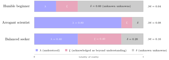
Assumption B.12.4 (Equal cost). Reading \(\nabla\mathcal{M}\) as the direction of fastest growth uses the Euclidean metric on the \((\lambda, \xi)\) plane, which amounts to assuming that a unit of effort buys equal increments of \(\lambda\) and of \(\xi\). If one unit of \(\xi\) cost \(c\) times the effort of one unit of \(\lambda\), the return per unit of effort would be \(\xi\) on Pattern and \(\lambda/c\) on Mystery; Mystery would then be the better investment only when \(\lambda/c > \xi\), which for \(c > 1\) can fail even where \(\xi\) is the weaker dimension. The model adopts equal cost throughout this section, and every reading of the form “your next step is reverence” rests on it.
Results and Proofs
Why a product? The three criteria below describe the shape Lucidity requires, and the product is the only function that meets all three.
Proposition B.12.5 (Uniqueness of the product). Let \(f\) be a smooth function on \((0,1)^2\), extended by continuity to the closed square, that meets three criteria:
Dual-face necessity. \(f(\lambda, 0) = f(0, \xi) = 0\): lacking either face, Lucidity is zero.
Symmetry. \(f(\lambda, \xi) = f(\xi, \lambda)\): Pattern and Mystery hold equal ontological status (Postulate 3).
Linear reciprocity. \(\partial f/\partial\lambda = \xi\) and \(\partial f/\partial\xi = \lambda\): the marginal return on advancing in one dimension exactly equals the current value of the other.
Then \(f = \lambda\xi\).
Suppose \(f(\lambda, \xi) = f(\xi, \lambda)\) and \(\partial f/\partial\lambda = \xi\). Then \(f = \lambda\xi + g(\xi)\). By symmetry, \(\partial f/\partial\xi = \lambda\), so \(f = \lambda\xi + h(\lambda)\). Hence \(g(\xi) = h(\lambda) = C\). Annihilation, extended by continuity to the corner, gives \(f(0,0) = 0\), so \(C = 0\), i.e. \(f = \lambda\xi\).
Why not a mean. The arithmetic mean fails the first criterion: a pure Logonaut would have \(\lambda/2 > 0\) “Lucidity,” which is wrong. The strongest competitor is the harmonic mean \(H = 2\lambda\xi/(\lambda+\xi)\). It meets the first two criteria, and its gradient \(\nabla H = \frac{2}{(\lambda+\xi)^2}(\xi^2, \lambda^2)\) also points toward the weaker dimension, so its qualitative ethical conclusions match the product’s; it fails the third. Table 16 lists the marginal returns of four candidate operators, and only the product’s depends purely on the other dimension1. The two are simply related: \(H = 2\mathcal{M}/(\lambda+\xi)\), the product divided by total awareness and multiplied by two. That extra normalization step destroys linear reciprocity without yielding any philosophical advantage.
| Function | Marginal return \(\partial\mathcal{M}/\partial\lambda\) | Depends on |
|---|---|---|
| \(\lambda\xi\) (product) | \(\xi\) | other only |
| \(\lambda^2\xi^2\) | \(2\lambda\xi^2\) | both |
| \(\sqrt{\lambda\xi}\) | \(\frac{1}{2}\sqrt{\xi/\lambda}\) | ratio of both |
| \(\frac{2\lambda\xi}{\lambda+\xi}\) (harmonic) | \(\frac{2\xi^2}{(\lambda+\xi)^2}\) | nonlinear mix of both |
Strictly, symmetry, annihilation, and a marginal return depending on the other dimension alone admit the family \(a\lambda\xi\) with \(a > 0\); the coefficient \(a = 1\) is a normalization choice, written into \(\partial\mathcal{M}/\partial\lambda = \xi\), and it is also what makes \(\mathcal{M}(1,1) = 1\). The product is therefore unique up to a constant multiple. A number makes this concrete: with Mystery-awareness at \(\xi = 0.6\), each unit of Pattern improvement yields exactly \(0.6\) units of Lucidity gain. That is the full content of linear reciprocity.
Theorem B.12.6 (Gradient Theorem). \[\begin{equation} \label{eq:gradient-theorem} \nabla\mathcal{M} = \left(\frac{\partial(\lambda\xi)}{\partial\lambda},\; \frac{\partial(\lambda\xi)}{\partial\xi}\right) = (\xi,\; \lambda) \end{equation}\]
Direct partial differentiation: \(\partial(\lambda\xi)/\partial\lambda = \xi\), \(\partial(\lambda\xi)/\partial\xi = \lambda\).
Corollary B.12.7 (Mutual bootstrapping). An agent’s marginal return on advancing in Pattern equals its current depth in Mystery, and vice versa.
\(\partial\mathcal{M}/\partial\lambda = \xi\) means that if \(\xi \approx 0\), then no matter how much \(\lambda\) increases, \(\mathcal{M}\) barely grows. That is: understanding without Mystery-awareness is spinning in place. The gradient identity is exact; the reading of it offered here is an interpretation of that identity, which is why this is graded as a demonstration rather than a proof.
Corollary B.12.8 (Balance is optimal at fixed richness). For fixed \(r\), \(\mathcal{M}\) attains its maximum \(r^2/2\) at \(\theta = \pi/4\), that is, \(\lambda = \xi\), perfect balance.
By Equation (eq:lucidity-polar), \(\mathcal{M} = (r^2/2)\sin(2\theta)\), and on \((0, \pi/2)\) the factor \(\sin(2\theta)\) has its unique maximum \(1\) at \(\theta = \pi/4\).
Figure 71 plots this curve for several values of \(r\).
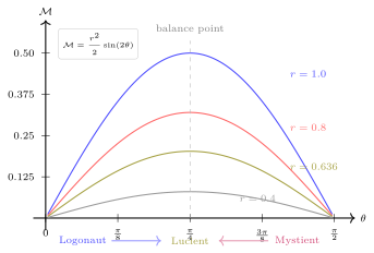
Corollary B.12.9 (Half-lucidity ceiling). Measuring richness by the Euclidean norm and fixing it at \(r = 1\), a balanced agent has:
\[\begin{equation} \label{eq:half-lucidity} \mathcal{M}_{\max}(r=1) = \frac{1}{2} \end{equation}\]
From Equation (eq:lucidity-polar), \(\mathcal{M}_{\max} = r^2/2\). At \(r = 1\) this gives \(1/2\). By T1, \(\lambda, \xi < 1\) so \(r < \sqrt{2}\), hence \(\mathcal{M} < 1\). Under ideal conditions (perfect balance, unit richness), Lucidity is exactly \(1/2\).
This ceiling fixes only \(r\) and stands on a different constraint surface from the ceiling under the three-zone normalization (Corollary B.12.11); see Table 15 and “Scope and limits” at the end of this section.
Corollary B.12.10 (\(\pi/2\) multiplier). At equal ontological richness \(r\), a perfectly balanced agent (\(\theta = \pi/4\)) has \(\pi/2\) times the mean Lucidity of an agent whose \(\theta\) is uniformly distributed on \((0, \pi/2)\) at that same \(r\).
Averaging \(\mathcal{M}\) uniformly over all orientations at fixed \(r\): \[\langle\mathcal{M}\rangle_\theta = \frac{2}{\pi}\int_0^{\pi/2} \frac{r^2}{2}\sin(2\theta)\,d\theta = \frac{r^2}{\pi}\] Thus \(\mathcal{M}_{\max} / \langle\mathcal{M}\rangle = (r^2/2)/(r^2/\pi) = \pi/2\).
Corollary B.12.11 (Total awareness is a ceiling, not a measure). Total awareness \(\lambda + \xi\) sets an upper bound on Lucidity but does not determine its value.
By the AM-GM inequality1: \(\lambda\xi \leq (\lambda + \xi)^2/4\), with equality if and only if \(\lambda = \xi\). Therefore, for fixed total awareness \(S = \lambda + \xi\):
\[\begin{equation} \mathcal{M} = \lambda\xi \leq \frac{S^2}{4} = \frac{(1-\delta)^2}{4} \end{equation}\]
Equality holds at \(\lambda = \xi = S/2\) (perfect balance). Because Definition B.12.3 forces \(S = 1 - \delta < 1\), this ceiling is strictly below \(1/4\), and it, rather than the unconstrained \(1/2\) of Corollary B.12.9, is the ceiling that binds under the three-zone normalization.
Proposition B.12.12 (Optimal reallocation under the normalization). This is the claim of B.1.4 that the optimal reallocation direction favors the weaker dimension. Hold \(\delta\), and so \(S = \lambda + \xi\), fixed, and move an amount \(t\) of awareness from \(\lambda\) to \(\xi\): \[\frac{d}{dt}\Big[(\lambda - t)(\xi + t)\Big]_{t=0} = \lambda - \xi.\] The derivative is positive exactly when \(\lambda > \xi\), so shifting awareness toward the weaker dimension raises \(\mathcal{M}\), and it keeps doing so until \(\lambda = \xi\), where the derivative vanishes at the balanced maximum of Corollary B.12.11. The exchange of one unit for one unit is the equal-cost assumption again.
Corollary B.12.13 (The smaller factor bounds Lucidity). \(\mathcal{M} \leq \min(\lambda, \xi)\). For fixed \(\delta > 0\) the bound is never attained; it becomes tight only in the limit \(\delta \to 0\) with the larger factor approaching \(1\).
By T1 the larger factor is below \(1\), so \(\mathcal{M} = \min(\lambda, \xi) \cdot \max(\lambda, \xi) < \min(\lambda, \xi)\).
Worked Example
One worked example puts the results above on a single set of numbers.
Mathematical portraits of the three archetypes. Projecting Lucidosophy’s three archetypal images (§IV) onto the \((\lambda, \xi)\) plane, with all three at the same total awareness \(\lambda + \xi = 0.9\):
| Archetype | \(\lambda\) | \(\xi\) | \(r\) | \(\theta\) | Total awareness | Lucidity \(\mathcal{M}\) | Gradient direction |
|---|---|---|---|---|---|---|---|
| Logonaut | \(0.80\) | \(0.10\) | \(0.806\) | \(7.1°\) | \(0.90\) | \(0.080\) | \(\to\) increase \(\xi\) |
| Mystient | \(0.10\) | \(0.80\) | \(0.806\) | \(82.9°\) | \(0.90\) | \(0.080\) | \(\to\) increase \(\lambda\) |
| Lucient | \(0.45\) | \(0.45\) | \(0.636\) | \(45.0°\) | \(0.90\) | \(0.203\) | perfectly balanced |
The three archetypes are plotted in the \(\lambda\)-\(\xi\) plane in Figure 72.
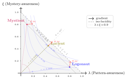
All three face the same amount of reality (total awareness \(0.9\)) and leave the same blind spot (\(\delta = 0.1\)). Yet the Lucient’s Lucidity is \(2.5\) times that of either the Logonaut or the Mystient, solely because of balance. The Logonaut and Mystient even have higher ontological richness (\(r = 0.806\)) than the Lucient (\(r = 0.636\)): they have traveled further in their respective directions, but the further they go, the more severely the polar balance factor \(\sin(2\theta)/2\) penalizes them. The iso-lucidity curves (\(\mathcal{M} = c\) hyperbolas) in the diagram make this vivid: the Logonaut and Mystient sit on a lower iso-lucidity curve, while the Lucient sits on a higher one.
The polar decomposition splits Lucidity into \(r^2\) (how much is invested) and \(\sin(2\theta)/2\) (how balanced the investment is), and everything the Logonaut and Mystient lose, they lose on the second factor: their richness has not shrunk, yet the Lucidity they extract from it has. The example is also an instance of Proposition B.12.12: holding \(S = 0.9\) fixed and shifting the Logonaut’s awareness step by step toward Mystery raises Lucidity all the way to the Lucient, where it reaches the ceiling \(S^2/4 \approx 0.203\) of Corollary B.12.11.
The Gradient Theorem locates each archetype’s steepest direction of gain (the gradient arrows in the diagram): the Logonaut’s next step is reverence (\(\nabla\mathcal{M}\) points nearly straight up, toward increasing \(\xi\)); the Mystient’s next step is analysis (\(\nabla\mathcal{M}\) points nearly straight right, toward increasing \(\lambda\)); the Lucient’s gradient runs along the \(45°\) diagonal, advancing equally in both dimensions. The same two movements appear in the three-archetype relationship diagram of Chapter §IV, read there from Lucient’s side: what Lucient learns from Logonaut is what Mystient must acquire, and what Lucient learns from Mystient is what Logonaut must acquire.
The gradient vector field. The following figure (Figure 73) displays \(\nabla\mathcal{M} = (\xi, \lambda)\) across the entire \(\lambda\)-\(\xi\) plane. Each arrow indicates the optimal growth direction for an agent at that position.
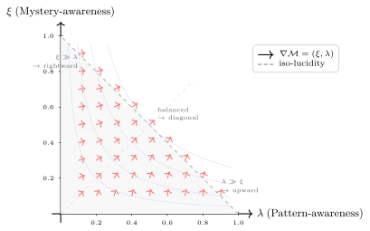
Twenty-five representative thinkers are located in the \(\lambda\)-\(\xi\) plane in Figure 74.
Interpretation
In everyday terms. Think of a mountain guide. She knows the routes and the patterns of the weather, which stands for Pattern-awareness, her grasp of Pattern (structure that can be stated and derived). She also accepts that the mountain always holds things no forecast can call, and leaves room for them, which stands for Mystery-awareness, her openness to Mystery (the part of reality that concepts do not close over). Lucidity measures how far she has both at once: if either is missing, lucidity falls toward zero, and what one more step on either side buys depends on how much of the other she already has. So a guide who knows every route by heart but never makes room for surprise gains more from spending her next hour learning respect for the mountain than from memorizing one more route, provided that an hour buys equal progress on either side. With her total attention fixed, lucidity is highest when the two are even.
The gradient as ethical direction. Bridge Axiom E4 says “choose Lucidity.” The Gradient Theorem, read under the equal-cost assumption (Assumption B.12.4), tells you how: your current weakness is where your next unit of effort yields the highest return. A scientist’s next step is reverence; a contemplative’s next step is logic; both are optimizing their own Lucidity. Where the return is highest is a calculus fact derived from the partial derivative of a product; that you ought to travel toward it comes from E4. The return in question is a return in Lucidity, which worldly return does not track. A supremely rational scientist with high \(\lambda\) and \(\xi\) near zero may achieve enormous worldly success (wealth, reputation, discoveries), and Lucidosophy’s mathematics does not deny it; what it says is that this scientist’s lucid integration of the whole of reality is near zero. They have comprehended reality’s analyzable portion but remain blind to its unanalyzable depths (finitude, meaning, reverence). What the Gradient Theorem tells them is: “your next unit of life-energy, if devoted to facing the depths you have been avoiding, will yield far greater Lucidity than publishing one more paper.”
Multiplication measures integration. In thermodynamics, free energy is \(F = U - TS\): order and entropy compete. In dialectics, thesis and antithesis oppose. Most everyday intuition uses addition: “I’ve learned some Pattern and experienced some Mystery, so I’m more lucid.” \(\mathcal{M} = \lambda \cdot \xi\) is multiplication: Pattern and Mystery cooperate. Zeroing out either destroys the whole, and unilateral growth while neglecting the other yields a Lucidity return per unit equal to the neglected factor, which is almost nothing when that factor is near zero. Addition measures how much of reality you cover; multiplication measures how much you integrate. The unconscious zone \(\delta\), for its part, is a structural blind spot that cannot be walked off like unexplored territory: no matter how learned or how reverent, there is always something you do not even know you do not know. Even under ideal conditions the product on the Euclidean level set of unit richness caps Lucidity at \(1/2\) (Corollary B.12.9), and under the three-zone normalization the ceiling is lower still (Corollary B.12.11). The old image of paired lights, sun and moon, says the same: half light, half dark.
Insights
In this model, leaning toward Pattern and leaning toward Mystery are the same imbalance in opposite directions, at equal cost. An engineer may think the person who only reveres is muddled, and a contemplative may think the person who only analyzes is shallow. Swap their shares, so that what one has in Pattern the other has in Mystery, and the model gives them exactly the same lucidity. The symmetry comes from a criterion the model adopts, that Pattern and Mystery hold equal standing; granting it, neither of two people in mirror positions has reason to think the other is further from lucidity.
If strengthening the weaker side costs far more than strengthening the stronger one, the best next step may still lie on the stronger side. The advice “move toward your weaker side” assumes that an hour of effort buys equal progress on either side. For a skilled analyst who finds an hour of quiet contemplation far harder than an hour of derivation, that assumption fails. If each step on the weaker side costs some multiple of a step on the stronger side, and that multiple exceeds the ratio of the stronger side’s current level to the weaker side’s, then the next hour spent on Pattern buys more lucidity, even though Mystery is the side where that analyst is weaker. Before acting on the advice, estimate what each side will cost.
The advice “move toward your weaker side” is sturdier than the uniqueness of the product. The product’s uniqueness (Proposition B.12.5) is bought by the third criterion, linear reciprocity, which is adopted on grounds of simplicity. Yet the gradient of the strongest competitor, the harmonic mean, \(\frac{2}{(\lambda+\xi)^2}(\xi^2, \lambda^2)\), likewise has its larger component on the weaker dimension (compare Table 16 and B.13). A reader who rejects linear reciprocity therefore still reaches the same qualitative direction under the equal-cost assumption (Assumption B.12.4); what changes with the operator is the value of the ceilings and the exact angle of the gradient.
Lucidity always stays below your weaker side, however far the stronger side goes. Corollary B.12.13 gives \(\mathcal{M} < \min(\lambda, \xi)\), since the larger factor is below \(1\) by T1. The Gradient Theorem (Theorem B.12.6) says which next step pays best; this corollary says how high the whole can rise: the weaker dimension sets a ceiling, and accumulation on the stronger dimension can only bring lucidity closer to it. The bound is pure algebra and does not depend on the equal-cost assumption.
With total awareness held fixed, shifting some attention from your strength to your weakness lowers the strength and raises your lucidity. By Proposition B.12.12, under the three-zone normalization with \(S = \lambda + \xi\) fixed, moving awareness from \(\lambda\) to \(\xi\) changes \(\mathcal{M}\) at rate \(\lambda - \xi\), positive while \(\lambda > \xi\), and the gain continues up to \(\lambda = \xi\). Since \(\lambda\) and \(\xi\) are shares of one agent’s attention, this growth faces no additional reality; it redistributes attention. The one-for-one exchange still rests on the equal-cost assumption.
Turning one unknown unknown into acknowledged Mystery raises the ceiling on lucidity exactly as much as turning it into understood Pattern. By Corollary B.12.11, under the three-zone normalization \(\mathcal{M} \leq S^2/4 = (1-\delta)^2/4\); the ceiling depends only on total awareness \(S\) and is symmetric in \(\lambda\) and \(\xi\). Shrinking the unconscious zone \(\delta\) therefore has two routes that count equally toward the ceiling: understanding something, or recognizing it as something you cannot understand. Growth then splits into two tasks: balance (adjusting \(\theta\) to approach the current ceiling) and widening awareness (shrinking \(\delta\) to raise the ceiling itself). All of this holds within the modeling convention of Definition B.12.3.
Interpretations and Illustrations
The material below uses the model as an interpretive lens. The names of the seven regions, the coordinates of historical figures (Figure 74 places twenty-five thinkers on the \(\lambda\)-\(\xi\) plane), and the life-course curves are the author’s readings; they show which positions the model can accommodate and supply no evidence for any result of this section.
The results above say only how the product rewards balance. A reader will also want to see what that reward looks like on actual people: which modes of being sit next to each other, which historical positions mirror each other, how one person’s lucidity rises and falls over a life. This material answers those questions, and in doing so it tests the model’s resolving power: a model that could not hold both Descartes and Rumi would be too narrow, and one that ranked everyone alike would be empty. What follows, in order: a table naming positions on the simplex, a scatter of twenty-five thinkers on the plane, the same thinkers redrawn by archetype angle, and five life-course curves. A reader may dispute any coordinate here. Doing so revises the author’s reading and leaves the theorems above untouched.
Canonical regions of the parameter simplex. The constraint \(\lambda + \xi + \delta = 1\) (\(\lambda, \xi > 0\) by T1 and \(\delta > 0\) for finite agents) defines the relative interior of the 2-simplex. We identify seven canonical subsets of this simplex that correspond to qualitatively distinct modes of being (see Chapter XV.4 for the full phenomenological analysis):
| Region | Name | Character |
|---|---|---|
| A | Deep Lucidity | High Pattern, high Mystery, small unaware zone. Simultaneous understanding and awe. Highest lucidity. |
| B | The Fog | Low Pattern, low Mystery, vast unaware zone. Balanced but nearly blind. Very low lucidity. |
| C | Crystal Tower | Very high Pattern, near-zero Mystery. Brilliant but brittle. Low lucidity despite vast knowledge. |
| D | Silent Valley | Near-zero Pattern, very high Mystery. Contemplative but voiceless. Low lucidity despite deep feeling. |
| E | Lucid Analyst | Pattern-led with genuine Mystery. Substantial lucidity. |
| F | Lucid Contemplative | Mystery-led with genuine Pattern. Substantial lucidity. |
| G | Sleepwalker | Near-zero Pattern, near-zero Mystery, vast unaware zone. Neither understands nor feels. Negligible lucidity. |
| Region | Name | \(\lambda\) | \(\xi\) | \(\delta\) | Formal characterization |
|---|---|---|---|---|---|
| A | Deep Lucidity | \(0.45\) | \(0.45\) | \(0.10\) | \(\lambda \approx \xi\), \(\delta \ll 1\): near the \(\mathcal{M}\)-maximum |
| B | The Fog | \(0.10\) | \(0.10\) | \(0.80\) | \(\lambda \approx \xi\), \(\delta \gg \lambda + \xi\): balanced but shallow |
| C | Crystal Tower | \(0.80\) | \(0.05\) | \(0.15\) | \(\lambda \gg \xi\), \(\delta\) moderate: Pattern-dominated |
| D | Silent Valley | \(0.05\) | \(0.80\) | \(0.15\) | \(\xi \gg \lambda\), \(\delta\) moderate: Mystery-dominated |
| E | Lucid Analyst | \(0.60\) | \(0.25\) | \(0.15\) | \(\lambda > \xi > 0\), both non-negligible |
| F | Lucid Contemplative | \(0.25\) | \(0.60\) | \(0.15\) | \(\xi > \lambda > 0\), both non-negligible |
| G | Sleepwalker | \(0.05\) | \(0.05\) | \(0.90\) | \(\lambda \approx \xi \approx 0\), \(\delta \to 1\) |
Note: Regions C and D have identical \(\mathcal{M}\) (\(= 0.040\)) by the commutativity of multiplication; similarly E and F (\(= 0.150\)). The product structure \(\mathcal{M} = \lambda\xi\) is symmetric in its arguments: Pattern-dominance and Mystery-dominance are mirror pathologies with identical lucidity deficits, and the decisive variable is always the smaller factor (Corollary B.12.13).
The numbers in both tables are representative points. Neighboring regions shade into one another, and the book draws no boundaries between them. The names come from the phenomenology of Chapter XV.4; the mathematics does two jobs, computing each region’s lucidity and naming the factor that holds it down. Regions B and G are the pair most worth reading together. Both sit on the balance line, and both have very low lucidity: balance sets what fraction of one’s awareness converts into lucidity, while the total amount of awareness (\(r\) in Equation (eq:lucidity-polar)) sets how much there is to convert. Regions A and B differ only in \(r\), which gives Chapter XV.4’s contrast between Deep Lucidity and The Fog a version one can compute.
Placing the thinkers. Putting historical figures on the plane shows how the product treats thinkers whose paths run in opposite directions. Descartes and Rumi, Kant and Zhuangzi sit on opposite sides of the balance line, and the product penalizes lopsidedness on either side alike, so mirror-image positions receive equal lucidity. The coordinates follow one reading rule. \(\lambda\) reflects how much of a person’s writings and public conduct consists of structure that can be stated, derived, and tested (systems, proofs, methods); \(\xi\) reflects where that person openly acknowledges the limit of what can be said (reverence, the apophatic way, facing finitude); \(\delta\) is what remains. The two decimal places only keep neighboring points apart on the chart. What can be taken seriously is relative position: who leans further toward Pattern than whom, who sits closer to the balance line. A reader who thinks someone is misplaced can move the point by the same rule and let the product compute the new lucidity; what changes is the author’s judgment, and the model stays as it is.
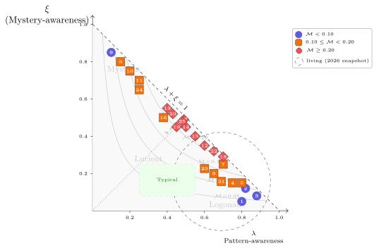
| # | Thinker | \(\lambda\) | \(\xi\) | \(\mathcal{M}\) | # | Thinker | \(\lambda\) | \(\xi\) | \(\mathcal{M}\) |
|---|---|---|---|---|---|---|---|---|---|
| 1 | Descartes | 0.80 | 0.05 | 0.040 | 11 | Zhuangzi | 0.25 | 0.70 | 0.175 |
| 2 | Spinoza | 0.82 | 0.12 | 0.098 | 12 | Plato | 0.60 | 0.35 | 0.210 |
| 3 | Gödel | 0.88 | 0.08 | 0.070 | 13 | Buddha | 0.40 | 0.55 | 0.220 |
| 4 | Aristotle | 0.75 | 0.15 | 0.113 | 14 | Wittgenstein | 0.50 | 0.45 | 0.225 |
| 5 | Einstein | 0.80 | 0.15 | 0.120 | 15 | Nietzsche | 0.55 | 0.40 | 0.220 |
| 6 | Confucius | 0.65 | 0.20 | 0.130 | 16 | Qu Yuan | 0.38 | 0.50 | 0.190 |
| 7 | Kant | 0.70 | 0.25 | 0.175 | 17 | Socrates | 0.49 | 0.49 | 0.240 |
| 8 | Laozi | 0.15 | 0.80 | 0.120 | 18 | Da Vinci | 0.70 | 0.29 | 0.203 |
| 9 | Rumi | 0.10 | 0.85 | 0.085 | 19 | Wang Yangming | 0.45 | 0.45 | 0.203 |
| 10 | Meister Eckhart | 0.20 | 0.75 | 0.150 | 20 | Gandhi | 0.43 | 0.52 | 0.224 |
| 21 | Musk | 0.69 | 0.157 | 0.108 | 22 | Jobs | 0.65 | 0.32 | 0.208 |
| 23 | Hawking | 0.60 | 0.227 | 0.136 | 24 | Mother Teresa | 0.25 | 0.65 | 0.163 |
| 25 | Mandela | 0.48 | 0.48 | 0.230 |
Philosophical interpretation. Several points can be read from this chart:
A different view of the thinkers. Polar coordinates separate two questions: \(r\) measures how much awareness a person has, and \(\theta\) measures which side it leans toward (Equation (eq:lucidity-polar)). On the \(\lambda\)-\(\xi\) plane the two are tangled; on the \(\theta\) axis the effect of balance shows on its own. The \(\lambda\)-\(\xi\) chart above crowds many thinkers into the corners of the feasible triangle. Switching to Lucidity–archetype-angle coordinates (\(\mathcal{M}\) vs \(\theta\)), twenty of them (numbers 1–20) reveal a strikingly different distribution (Figure 75):
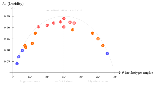
What this view reveals. Thinkers who were crowded into two corners of the \(\lambda\)-\(\xi\) chart now spread naturally along the \(\theta\) axis: Logonaut zone (left), Lucient zone (center), Mystient zone (right). The most striking pattern is the hill shape: high-lucidity markers cluster almost entirely in the central band \(\theta = 30°\)–\(55°\), forming a “Lucidity highland.” Socrates (17) sits precisely at the \(\theta = 45°\) peak, a direct manifestation of the balance factor \(\sin(2\theta)/2\). The envelope is the normalized ceiling, the supremum of \(\mathcal{M}\) at angle \(\theta\) under \(\lambda + \xi < 1\). On the boundary \(\lambda + \xi = 1\) we have \(r(\cos\theta + \sin\theta) = 1\), so \(r^2 = 1/(1 + \sin 2\theta)\), and Equation (eq:lucidity-polar) gives \[\mathcal{M}_{\max}(\theta) = \frac{\sin 2\theta}{2(1 + \sin 2\theta)},\] which peaks at \(1/4\) at \(\theta = 45°\) (Corollary B.12.11 with \(S \to 1\)). It is the three-zone counterpart of the unconstrained \(r = 1\) curve of Corollary B.12.9, whose peak of \(1/2\) would lie off this chart. Several thinkers sit close to it: Socrates at \(0.240\) against \(0.25\), Da Vinci (18) at \(0.203\) against \(0.207\). The closeness is a fact about the assignments, which leave these figures only a small unconscious zone (\(\delta = 0.02\) and \(0.01\)).
Note also the symmetry: Kant (7, \(\theta \approx 20°\)) and Zhuangzi (11, \(\theta \approx 70°\)) are nearly symmetric about \(45°\), with identical Lucidity. Different paths through reason and mystery can lead to the same level of lucidity.
One caution in reading this chart. Every point’s lucidity is computed from the author’s coordinates by the same product, so the hill shape is the shape of the formula and cannot count as independent support for balance. Its use is to show at a glance whom the author judged balanced and whom lopsided; disagreement with those judgments belongs here.
Lucidity across life stages and professions. Lucidity shifts with life stage and vocational path. The charts so far are snapshots; these curves add time. They are qualitative sketches fitted to no data. Each shape has a reading in the master equation (B.14): socialization reads as a rise in the dissipation rate \(\gamma\), sustained study or meditation as a growth rate \(\alpha\) kept up, and late-life awareness of finitude (B.8) as a rise in \(\xi\) that moves the balance angle \(\theta\). Read the curves for the differences among their shapes; the heights on the vertical axis are illustrative. The following chart (Figure 76) shows typical Lucidity trajectories for different life courses:
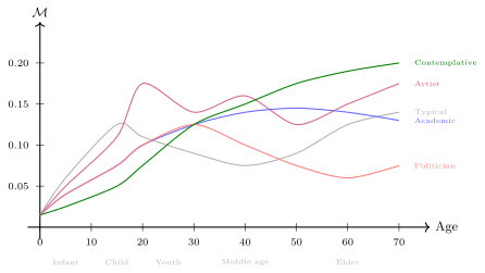
Insights.
The five curves share one feature. Every rising stretch has something steadily feeding \(\lambda\) or \(\xi\) (curiosity, creative work, study, meditation, or late-life awareness of finitude); most falling stretches are that feeding crowded out by something else (the demands of socialization, the confidence that comes with power). This is B.14’s “for a single agent, obscuration is the default” at the scale of a life.
Scope and limits
What buys uniqueness. The uniqueness of Proposition B.12.5 is bought by the third criterion, linear reciprocity, which is adopted on grounds of simplicity (see B.1.4). Under the first two criteria alone the harmonic and geometric means remain candidates; the qualitative conclusions survive, while the quantitative ones (ceiling values, gradient directions) change (see B.13). Separability in polar coordinates gives no further reason: every positively homogeneous operator factors into a power of \(r\) times a function of \(\theta\), the harmonic mean included (\(H = r \cdot \sin(2\theta)/(\cos\theta + \sin\theta)\)), so it does not tell the product apart from its rivals.
The normalization is a convention. Definition B.12.3 normalizes reality to \(1\); this is a modeling convention and makes no metaphysical assertion. It assumes that “the totality of reality” can be treated as a finite whole and partitioned among three zones. This is natural for proportional analysis (“how much do you understand?”), but it also implies that \(\lambda\) and \(\xi\) do not overlap, i.e., that “understanding” and “reverence” point to disjoint domains. If some experiences involve both at once (e.g., a mathematician confronting a profound proof), the normalized model treats this as a boundary effect between two zones and posits no fourth zone. This is a simplification.
\(\delta > 0\) is stronger than the Boundary Theorem. Definition B.12.3 renders Postulate 6 as \(\delta > 0\), which excludes points such as \((0.6, 0.6)\) that T1 allows. The dependence runs one way: T1, which says that full lucidity is unreachable, is proved in B.1.4 from \(\lambda < 1\) and \(\xi < 1\) without any \(\delta\), while the stronger stipulation \(\delta > 0\) implies its upper bound and more (\(\mathcal{M} < 1/4\) by Corollary B.12.11).
Equal cost. Every reading of the gradient as “where to step next” rests on Assumption B.12.4; when effort costs differ between the two dimensions, the best investment can lie away from the weaker one.
Every ceiling names its surface. The value \(1/2\) belongs to these two choices, the Euclidean norm and the level \(r = 1\); neither is forced, and on the whole domain \((0,1)^2\) that T1 allows, the supremum of \(\lambda\xi\) is \(1\), approached as both factors tend to \(1\). This ceiling is unconstrained: it fixes only ontological richness \(r\) and lets \(\lambda + \xi\) run as high as \(\sqrt{2}\). It must therefore never be quoted on its own. Under the three-zone normalization of Definition B.12.3, where \(\lambda + \xi + \delta = 1\) with \(\delta > 0\), the binding ceiling is the tighter one of Corollary B.12.11, \(\mathcal{M} \leq S^2/4 < 1/4\). The two are ceilings on different constraint surfaces, and every statement about the ceiling on Lucidity must say which surface it stands on. Table 15 sets the ceilings side by side.
The \(\pi/2\) multiplier depends on the measure. The multiplier depends on the averaging measure. Averaging instead along a segment of fixed total awareness \(\lambda + \xi = S\), uniformly in \(\lambda\), gives \(\langle\mathcal{M}\rangle = \frac{1}{S}\int_0^S \lambda(S - \lambda)\,d\lambda = S^2/6\) against the balanced \(S^2/4\), a multiplier of \(3/2\). Corollary B.12.10 stands on the unconstrained surface of fixed \(r\); under the three-zone normalization of Definition B.12.3 the balanced point at fixed \(r\) is feasible only for \(r < 1/\sqrt{2}\).
B.13 · Optimality of the Dual Face
Question: Why should Reality have two faces, and how many does the product model favor?
Requires: The product structure of B.12; the AM-GM inequality.
Yields: Within the product model, \(n = 2\) gives the highest lucidity ceiling (Theorem B.13.2), also under a linear constraint (Proposition B.13.3), and a comparison with the other candidate operators.
Postulate 3 asserts that Reality has two faces. Why exactly two, not one, three, or five? This section shows that within the product-based Lucidity model developed above, \(n = 2\) yields the highest possible Lucidity ceiling among all \(n \geq 2\) non-trivial ontological structures. This result provides structural support for Postulate 3’s dual-aspect claim, but it is a theorem about the model, not a proof that reality must have exactly two faces. Its force depends on accepting the product functional and the quadratic richness constraint as well-motivated modeling choices (see B.1.4 and B.12 for the justification of both).
Setup
Definition B.13.1 (\(n\)-face lucidity). Generalize Postulate 3: suppose Reality has \(n\) faces, with the agent’s awareness of each face being \(x_i \in (0,1)\), \(i = 1, \ldots, n\). Extending the product structure of Equation (eq:lucidity-product):
\[\begin{equation} \label{eq:n-face-lucidity} \mathcal{M}_n = \prod_{i=1}^{n} x_i \end{equation}\]
Constraint: total ontological richness \(\sum_{i=1}^n x_i^2 = r^2\) is fixed.
Results and Proofs
Theorem B.13.2 (Dual-face optimality). Let each \(x_i < 1\), as T1 requires, and fix \(r\) with \(0 < r < \sqrt{2}\) (the range in which the balanced two-face allocation is feasible). Then, for \(n \geq 2\), the maximum of \(\mathcal{M}_n\) is greatest when \(n = 2\).
Apply the AM-GM inequality to \(x_1^2, \ldots, x_n^2\): under the constraint \(\sum x_i^2 = r^2\), \(\prod x_i^2 \leq (r^2/n)^n\), with equality exactly when \(x_1 = x_2 = \cdots = x_n = r/\sqrt{n}\). This point satisfies \(x_i < 1\), since \(r < \sqrt{2} \leq \sqrt{n}\). Substituting:
\[\begin{equation} \mathcal{M}_n^* = \left(\frac{r}{\sqrt{n}}\right)^n = \frac{r^n}{n^{n/2}} \end{equation}\]
To show \(\mathcal{M}_n^*\) is strictly decreasing in \(n\) for fixed feasible \(r\) (\(n \geq 2\)), examine the ratio of consecutive ceilings: \[\frac{\mathcal{M}_{n+1}^*}{\mathcal{M}_n^*} = r \cdot \frac{n^{n/2}}{(n+1)^{(n+1)/2}}.\] The hypothesis \(r < \sqrt{2}\) comes from T1: with each \(x_i < 1\), the balanced allocation \(x_i = r/\sqrt{2}\) at \(n = 2\) is feasible only for \(r < \sqrt{2}\). Moreover \((n+1)^{(n+1)/2}/n^{n/2} = \sqrt{n+1}\,(1 + 1/n)^{n/2} \geq \sqrt{3} > \sqrt{2} > r\), so for \(n \geq 2\) the ratio is strictly less than \(1\), and \(\mathcal{M}_n^*\) is strictly decreasing. The cap \(x_i < 1\) carries the argument: without it, the ratio at \(n = 2\) is \(2r/3^{3/2}\), which exceeds \(1\) once \(r > 3\sqrt{3}/2 \approx 2.60\), and three faces would then beat two.
Explicit values (the table takes \(r = 1\)):
| Number of faces \(n\) | Lucidity ceiling \(\mathcal{M}_n^*\) |
|---|---|
| \(1\) | excluded(no duality; the only point \(x_1 = 1\) violates T1) |
| \(2\) | \(0.500\)(Highest non-trivial ceiling) |
| \(3\) | \(0.192\) |
| \(4\) | \(0.063\) |
| \(5\) | \(0.018\) |
\(n = 1\) (one face) is excluded on philosophical grounds: a single face offers nothing to contrast or integrate. Formally \(\mathcal{M}_1 = x_1 = r\), which at \(r = 1\) would require \(x_1 = 1\), outside the domain of T1. \(n = 2\) (two faces) yields the highest admitted ceiling. From \(n = 2\) to \(n = 3\), the ceiling plummets by \(62\%\) at \(r = 1\); in general the drop is \(1 - 2r/3^{3/2} \approx 1 - 0.385\,r\) (Figure 77).
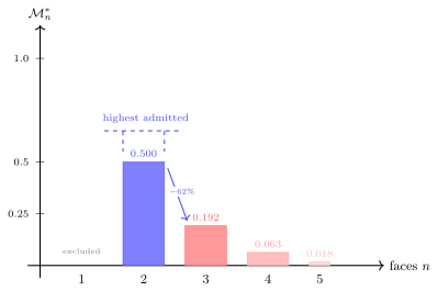
Proposition B.13.3 (Dual-face optimality under a linear constraint). Replace the quadratic constraint of Definition B.13.1 by the linear constraint \(\sum_{i=1}^n x_i = S\) with \(0 < S < 2\) (so that the balanced two-face point is feasible under T1). Then the ceiling of \(\mathcal{M}_n\) is \((S/n)^n\), and it is strictly decreasing in \(n\) for \(n \geq 2\): \(n = 2\) still yields the highest ceiling.
By the AM-GM inequality, \(\prod x_i \leq (S/n)^n\), with equality at \(x_i = S/n\). Moreover \((S/(n+1))^{n+1} < (S/n)^n\), because \(S < 2 < (n+1)(1 + 1/n)^n\).
Comparison with other operators. The product structure (\(\mathcal{M} = \lambda\xi\)) is the unique solution under the three criteria of Proposition B.12.5 (annihilation, symmetry, linear reciprocity). If one relaxes the third criterion, other operators become admissible. The following table compares the product against four alternatives: the harmonic mean, geometric mean, and minimum satisfy annihilation and symmetry but not linear reciprocity; the asymmetric weighted operator (\(a \neq 1/2\)) gives up symmetry as well:
| Product | Harmonic | Geometric | Minimum | Weighted | |
| \(\lambda\xi\) | \(\dfrac{2\lambda\xi}{\lambda+\xi}\) | \(\sqrt{\lambda\xi}\) | \(\min(\lambda,\xi)\) | \(\lambda^a\xi^{1-a}\) | |
| Gradient | \((\xi,\;\lambda)\) | complex* | \(\left(\dfrac{1}{2}\sqrt{\dfrac{\xi}{\lambda}},\;\dfrac{1}{2}\sqrt{\dfrac{\lambda}{\xi}}\right)\) | discontinuous | \((a\lambda^{a-1}\xi^{1-a},\ldots)\) |
| Symmetry | \(\checkmark\) | \(\checkmark\) | \(\checkmark\) | \(\checkmark\) | only if \(a = 1/2\) |
| Ceiling (\(\delta\!\to\!0\)) | \(1/4\) | \(1/2\) | \(1/2\) | \(1/2\) | \(0.529\) at \(a\!=\!2/3\) |
| Balanced seeker | |||||
| \(\lambda\!=\!\xi\!=\!0.4\) | \(0.160\) | \(0.400\) | \(0.400\) | \(0.400\) | \(0.400\) |
| Arrogant scientist | |||||
| \(\lambda\!=\!0.8,\;\xi\!=\!0.1\) | \(0.080\) | \(0.178\) | \(0.283\) | \(0.100\) | \(0.400\) |
| Imbalance penalty | |||||
| (ratio of above) | \(2.00\times\) | \(2.25\times\) | \(1.41\times\) | \(4.00\times\) | \(1.00\times\) |
| Mutual bootstrapping | exact | partial | partial | none | only if \(a\!=\!1/2\) |
| \(n\!=\!2\) optimal? | \(\checkmark\) | \(\checkmark\)§ | \(\checkmark\)§ | \(\checkmark\)§ | undefined§ |
*\(\nabla H = \bigl(2\xi^2/(\lambda+\xi)^2,\; 2\lambda^2/(\lambda+\xi)^2\bigr)\), symmetric but algebraically opaque.
At \(a = 2/3\) (asymmetric weighting toward Pattern); here \(0.8^{2/3} \cdot 0.1^{1/3} = (0.8^2 \cdot 0.1)^{1/3} = 0.4\), so the imbalance penalty vanishes exactly. Different \(a\) values yield different penalties.
“Exact” means \(\partial\mathcal{M}/\partial\lambda = \xi\): your marginal return on Pattern is your current Mystery-awareness. No other operator produces this clean reciprocity.
§Under \(\sum x_i^2 = r^2\), the \(n\)-ary minimum, harmonic mean and geometric mean satisfy \(\min_i x_i \leq H \leq G \leq \sqrt{\sum x_i^2/n} = r/\sqrt{n}\), with equality throughout at \(x_i = r/\sqrt{n}\); their common ceiling \(r/\sqrt{n}\) decreases in \(n\). The weighted operator has no canonical \(n\)-face form: the natural one, \(\prod x_i^{a_i}\) with \(\sum a_i = 1\), has ceiling \(r\prod a_i^{a_i/2}\), which depends on the weights and does not decrease with \(n\).
Interpretation
In everyday terms. Picture a cook with a fixed number of practice hours a week, preparing a dish that needs several skills at once: if any one skill is weak, the whole dish suffers. In this picture the fixed hours play the role of the model’s fixed total investment, each skill plays one face of Reality, and the quality of the dish plays lucidity (the product of the agent’s awareness of each face), so a zero on any face makes the whole product zero. A dish that needs only one skill has nothing to contrast, and the model sets it aside. Going from two skills to three thins each skill’s share of the hours, and once the shares are multiplied, the best the dish can reach falls steeply. In the product model, two faces is the number that gives the highest ceiling on lucidity.
A mathematical defense of Postulate 3. Within the product model above, among all structures with at least two faces, the two-face structure provides the most generous Lucidity ceiling. The ceiling \(\mathcal{M}_n^* = \exp\bigl(n\ln r - \tfrac{n}{2}\ln n\bigr)\) falls faster than exponentially in \(n\). The model contains no term that rewards complexity: the ceiling falls monotonically with \(n\), and \(n = 1\) is excluded for a philosophical reason (a single face has nothing to contrast), so \(n = 2\) is optimal among \(n \geq 2\) as the fewest faces that still leave a contrast.
The optimal non-trivial ontology. If one were to design a reality that is “comprehensible but not completely comprehensible” (structured enough that awakening is meaningful, yet opaque enough that complete awakening is impossible), then, measured by the product model, the optimal design is exactly a two-face structure. This does not mean other traditions’ ontological categories are “wrong”; they may describe different levels of unfolding.
Insights
When the total investment is fixed and the result multiplies the faces together, spreading the investment evenly across the faces gives the highest lucidity. A shop owner has a fixed number of working hours a week, and income depends on both making goods and selling them; if either is zero, income is zero. In the setting of this model, splitting the hours evenly between the two gives the largest product, and any lopsided split falls below the ceiling. The conclusion needs both conditions at once: a fixed total, and a result formed by multiplying the faces.
The more faces must be present at once, the larger the share of the best attainable lucidity each additional face takes away. A job counts as done only if several departments all do their part, and the total staff is fixed: going from two departments to three already lowers the best possible result, and going from three to four lowers it by a larger share than the step before. In this model this holds when the total is fixed and the faces are multiplied, comparing the highest lucidity each structure can reach. It is a conclusion about the model: it shows that product scoring favors the fewest faces that still leave a contrast, and it does not prove that Reality has exactly two faces.
In the product model, dual-face optimality depends on T1: if every face could be fully known, an agent with enough richness would prefer three faces. The proof of Theorem B.13.2 uses the cap \(x_i < 1\) at its last step, and that cap is what keeps the richness at \(r < \sqrt{2}\); drop it, and the ratio of successive ceilings at \(n = 2\) is \(2r/3^{3/2}\), which exceeds \(1\) once \(r > 3\sqrt{3}/2 \approx 2.60\), so three faces beat two. In this model, then, the two faces of Postulate 3 and “awareness of each face stays below \(1\)” belong together: bounded awareness is what makes two faces optimal across the whole feasible range.
Each additional face that must be present at once lowers the best Lucidity a fixed total investment can reach, and this cost of extra faces comes from holding the total fixed. By Equation (eq:n-face-ceiling) the ceiling is \(r^n/n^{n/2}\), which falls by \(62\%\) from \(n = 2\) to \(n = 3\) at \(r = 1\) (Table 21); replacing the quadratic constraint with a linear one leaves the conclusion intact (Proposition B.13.3). Under the per-face cap \(x_i < 1\) alone, with no fixed total, \(\sup \prod x_i = 1\) for every \(n\), and an extra face costs nothing.
All four symmetric operators deliver “balance beats imbalance”; what the product adds is a rule for the margin: how much one more step in Pattern is worth is set by how deep you already are in Mystery. In Table 22 the product, harmonic mean, geometric mean, and minimum agree on the three qualitative conclusions, and only the product satisfies \(\partial\mathcal{M}/\partial\lambda = \xi\) (the linear reciprocity of Proposition B.12.5). A reader who prefers another symmetric operator keeps the ethics of balance and loses only this exact marginal rule; the asymmetric weighted operator shows the other side, since in the table’s \(a = 2/3\) example the imbalance penalty vanishes, so giving up symmetry can take the ethics of balance with it.
Scope and limits
Constraint surface. Theorem B.13.2 uses the quadratic constraint \(\sum x_i^2 = r^2\) (fixed ontological richness), while Definition B.12.3 uses the linear normalization \(\sum x_i + \delta = 1\); the two are different constraint surfaces (see Table 15). The quadratic level set is chosen because it naturally generalizes to \(n\) dimensions and allows clean Lagrange-multiplier analysis; for the linear constraint see Proposition B.13.3. The numerical values in Table 21 assume the quadratic constraint.
Reach among symmetric constraints. The conclusion does not extend to every symmetric constraint: the box constraint \(x_i < 1\) alone gives \(\sup \prod x_i = 1\) for every \(n\).
Other symmetric operators. Readers who prefer another symmetric operator will find the three qualitative conclusions compared in Table 22 unchanged (balance beats imbalance, both dimensions are necessary, \(n = 2\) is optimal among \(n \geq 2\)). Conclusions that use the gradient, such as B.12’s direction of fastest growth, do not carry over as stated (the minimum has no gradient on the diagonal), and the quantitative results (ceiling values, gradient directions) will differ.
B.14 · The Four-Mode Master Equation
Question: How does lucidity evolve over time?
Requires: The basic notion of an ordinary differential equation; the polar form and ceilings of B.13.
Yields: The four-mode master equation, its steady state and stability, imbalance as self-dissipation (Proposition B.14.4), and the logistic time solution.
The four fundamental modes of Pattern from Chapter §II (dissipation, gradient, selection, feedback) are not merely a taxonomy. We propose a phenomenological model that synthesizes them into a single equation governing how Lucidity evolves over time. Each mode contributes one mathematical factor. This is a modeling choice informed by the prior sections, not a deduction from them.
Setup
Assumption B.14.1 (The master equation). The time evolution of Lucidity \(\mathcal{M}(t)\) is governed by:
\[\begin{equation} \label{eq:master-equation} \frac{d\mathcal{M}}{dt} = \underbrace{\alpha\mathcal{M}}_{\text{Feedback}} \cdot \underbrace{\left(1-\frac{\mathcal{M}}{K(\theta)}\right)}_{\text{Selection}} \cdot \underbrace{\sin(2\theta)}_{\text{Gradient}} \;-\; \underbrace{\gamma\mathcal{M}}_{\text{Dissipation}}, \qquad K(\theta) = \sin(2\theta) \end{equation}\]
where:
Feedback (\(\alpha\mathcal{M}\)): growth is proportional to current Lucidity: the more lucid, the faster you awaken. This is bootstrapping. \(\alpha > 0\) is the growth rate.
Selection (\(1-\mathcal{M}/K(\theta)\)): as \(\mathcal{M}\) approaches the ceiling \(K(\theta)\) available at angle \(\theta\), room for improvement vanishes. The ceiling comes from T1 and B.12: at fixed \(\theta\), \(\mathcal{M} = (r^2/2)\sin(2\theta) < \sin(2\theta)\), since \(r^2 = \lambda^2 + \xi^2 < 2\). At balance \(K(\pi/4) = 1\). \(K(\theta)\) is the boundary-ceiling row of Table 15: this master equation operates on the unnormalized \(\mathcal{M} \in [0,1]\), and under the three-zone normalization the binding ceiling is the table’s three-zone row (\(\mathcal{M} \leq S^2/4 < 1/4\), Corollary B.12.11).
Gradient (\(\sin(2\theta)\)): growth is fastest at balance angle \(\theta = \pi/4\); zero at pure Pattern (\(\theta = 0\)) or pure Mystery (\(\theta = \pi/2\)).
Dissipation (\(-\gamma\mathcal{M}\)): without sustained practice, Lucidity naturally decays, the cognitive analogue of the second law of thermodynamics. \(\gamma > 0\) is the dissipation rate.
The interplay of these four factors is shown in Figure 78.
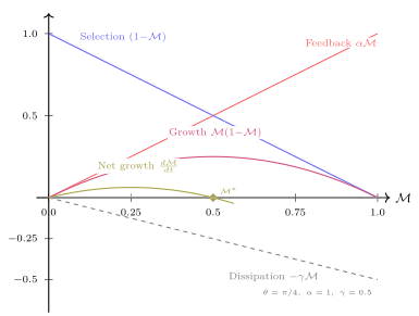
Results and Proofs
Steady state and stability.
Setting the right-hand side to zero gives the nonzero fixed point; its stability comes next.
Proposition B.14.2 (Steady state). Setting \(d\mathcal{M}/dt = 0\), assuming \(\mathcal{M} \neq 0\):
\[\begin{equation} \label{eq:steady-state} \alpha\left(1 - \frac{\mathcal{M}^*}{K(\theta)}\right)\sin(2\theta) = \gamma, \qquad\text{i.e.}\qquad \mathcal{M}^* = K(\theta)\left(1 - \frac{\gamma}{\alpha\sin(2\theta)}\right) \end{equation}\]
At optimal balance (\(\theta = \pi/4\), \(\sin(2\theta) = K = 1\)):
\[\begin{equation} \label{eq:steady-state-balanced} \mathcal{M}^* = 1 - \frac{\gamma}{\alpha} \end{equation}\]
Existence condition: \(\mathcal{M}^* > 0\) requires \(\alpha\sin(2\theta) > \gamma\); at balance, \(\alpha > \gamma\), i.e., growth rate must exceed dissipation rate.
Proposition B.14.3 (Stability). Write \(s = \sin(2\theta)\), \(\rho = \alpha s - \gamma\), and \(f(\mathcal{M}) = \alpha\mathcal{M}(1 - \mathcal{M}/K)s - \gamma\mathcal{M}\). With \(K = s\) this is \(f(\mathcal{M}) = \rho\mathcal{M} - \alpha\mathcal{M}^2\), so \(\mathcal{M}^* = \rho/\alpha\) and \(f'(\mathcal{M}) = \rho - 2\alpha\mathcal{M}\), giving \(f'(0) = \rho\) and \(f'(\mathcal{M}^*) = -\rho\). For \(\rho > 0\), \(0\) is unstable and \(\mathcal{M}^*\) is stable; for \(\rho < 0\), \(\mathcal{M}^* < 0\) is unphysical and \(0\) is stable. Since \(f(K) = -\gamma K < 0\), a trajectory starting in \([0, K)\) stays there, so \(\mathcal{M}\) never exceeds the static bound of B.13.
Half-lucidity and the dynamics. When \(\alpha = 2\gamma\), \(\mathcal{M}^* = 1/2\), the same value as the half-lucidity ceiling of B.12 (Figure 79); as the note after Table 15 says, the agreement comes from the choice of parameters and cannot count as independent evidence for \(1/2\).
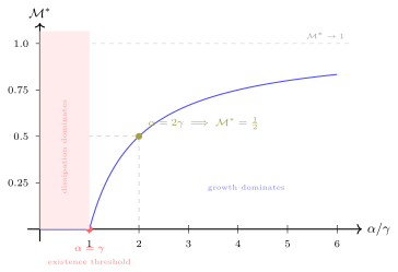
Imbalance as self-dissipation.
Rewriting the steady state shows what imbalance costs.
Proposition B.14.4 (Imbalance as self-dissipation). Rewriting Equation (eq:steady-state):
\[\begin{equation} \label{eq:effective-dissipation} \mathcal{M}^* = K(\theta)\left(1 - \frac{\gamma_{\text{eff}}}{\alpha}\right), \quad \text{where}\quad \gamma_{\text{eff}} = \frac{\gamma}{\sin(2\theta)} \end{equation}\]
When \(\theta \neq \pi/4\), \(\sin(2\theta) < 1\), so \(\gamma_{\text{eff}} > \gamma\), and the ceiling \(K(\theta)\) drops below \(1\) as well.
Conclusion. At steady state, imbalance acts as self-imposed additional dissipation, on top of a lowered ceiling. The equivalence holds for the steady state only: the full dynamics also change the ceiling \(K(\theta)\) and the time scale \(1/\rho\), so imbalance is not the same equation as a larger \(\gamma\). In this model a biased agent settles at a lower steady state, and past the critical angle \(\sin(2\theta_c) = \gamma/\alpha\) its Lucidity decays to zero.
Concretely: moderate imbalance (\(\theta = \pi/6\), Pattern/Mystery ratio of \(\sqrt{3}:1\)) increases effective dissipation by \(15\%\). Extreme imbalance (\(\theta = \pi/12\)) doubles it (Figure 80).
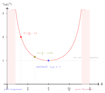
Time evolution.
Beyond the steady state, the master equation gives the full trajectory toward it.
Proposition B.14.5 (Logistic solution). Since \(f(\mathcal{M}) = \rho\mathcal{M}(1 - \mathcal{M}/\mathcal{M}^*)\), the master equation is a standard logistic equation at every angle with \(\rho = \alpha\sin(2\theta) - \gamma > 0\). Its solution, for \(\mathcal{M}_0 > 0\), is a sigmoid:
\[\begin{equation} \label{eq:sigmoid-lucidity} \mathcal{M}(t) = \frac{\mathcal{M}^*}{1 + \left(\dfrac{\mathcal{M}^*}{\mathcal{M}_0} - 1\right)e^{-\rho t}}, \qquad \rho = \alpha - \gamma \text{ at balance} \end{equation}\]
Three phases are visible:
Slow start: \(\mathcal{M} \approx \mathcal{M}_0 \, e^{\rho t}\) while \(\mathcal{M} \ll \mathcal{M}^*\), i.e., exponential awakening, but from a small base
Inflection: growth is fastest at \(\mathcal{M} = \mathcal{M}^*/2\), the moment of breakthrough
Asymptotic approach: \(\mathcal{M} \to \mathcal{M}^*\), i.e., diminishing returns, never quite arriving (from below when \(\mathcal{M}_0 < \mathcal{M}^*\); from above, without the sigmoid, when \(\mathcal{M}_0 > \mathcal{M}^*\))
\(e\) (Euler’s number) appears because the model is posed in continuous time: it is the natural base for the time scale \(1/\rho\) of both Lucidity growth and decay (Figure 81).
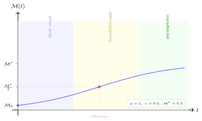
Phase portrait and time evolution. The following figure (Figure 82) shows the same dynamics in two panels. The left panel is the phase portrait, plotting \(d\mathcal{M}/dt\) directly as a function of \(\mathcal{M}\), so its zero-crossings are the fixed points; the right panel follows lucidity over time at the same three balance angles, and the fixed points of the left panel become the plateaus the curves approach:
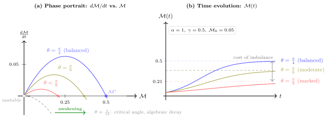
Interpretation
In everyday terms. Picture someone learning a foreign language. Leave it alone and the words already learned fade bit by bit: this plays the model’s dissipation, which is always at work and needs no one to push it. The more one knows, the more material one can read and the faster one learns, which plays feedback. The closer one gets to native level, the less room is left to improve, which plays the ceiling that selection sets. Balance stands for the mix of two kinds of awareness: command of rules that can be stated (Pattern), and a clear sense of where one’s grasp is still unsure (Mystery). The model’s conclusion: when growth outpaces forgetting, the level settles at a steady height; leaning toward one end acts, at that settled level, like extra forgetting, and past a certain limit everything learned drains away.
Synthesis of the four modes. The master equation does not merely juxtapose the four modes; it reveals their interaction: feedback drives growth, but selection sets the ceiling; gradient determines direction, but dissipation drags from behind. Understanding any single mode in isolation is insufficient; the dynamics of Lucidity is set by all four together.
For a single agent, obscuration is the default. The dissipation term \(-\gamma\mathcal{M}\) is always present; it requires no effort. The growth term \(\alpha\mathcal{M}(1-\mathcal{M}/K(\theta))\sin(2\theta)\) requires three active conditions simultaneously: an existing base of Lucidity (feedback), remaining room for improvement (selection), and deliberate balance (gradient).
The role of fundamental constants. Seeing \(e\) and \(\pi\) in an equation about lucidity, a reader may suppose the framework is invoking some deep constant. The table below shows where each enters the equation and separates the readings the equation forces from the interpretive ones. The master equation contains five fundamental mathematical objects, each of which Lucidosophy reads against its framework:
| Constant | Lucidosophy meaning |
|---|---|
| \(0\) | Complete obscuration, i.e., feedback’s absorbing state; a lone agent cannot restart from zero |
| \(1\) | Complete Lucidity, i.e., the unattainable ceiling set by T1; the ceiling \(K(\theta) = \sin 2\theta\) reaches it only at balance |
| \(2\) | The double-angle constant: \(\sin 2\theta = 2\sin\theta\cos\theta\) is the polar form of the product of two awarenesses (B.12), so it links to the Dual Face postulate (Postulate 3) through that product; it is a trigonometric constant, not a count of faces |
| \(e\) | Time scale of Lucidity growth and decay; it enters because the model is posed in continuous time |
| \(\pi\) | Enters through angle units (\(\theta = \pi/4\)); the balance advantage of intentional practice over random orientation (B.12) assumes a uniform average over \(\theta\) |
Three appearances of one number. By now a reader has probably noticed \(1/2\) recurring, and the image of sun and moon as half light, half dark at the close of B.12’s interpretation invites treating it as a meaningful number. This paragraph sets out where each appearance comes from. The number \(1/2\) appears in three places: B.12’s static geometry (\(r^2/2\)), B.14’s dynamical steady state (\(1 - \gamma/\alpha\) at balance when \(\alpha = 2\gamma\)), and the maximum-entropy point of a binary distribution in information theory (\(p = 1/2\)). Only the first is a derived ceiling; the second depends on the choice of parameters, and the third is a general property of any symmetric binary distribution. The three can sit side by side as an aid to memory, but they cannot count as independent confirmations of one another.
Insights
This model expects a long early stretch with little visible progress, and progress is fastest exactly halfway to the level where one will settle. Someone starts practicing calligraphy every day: for months little seems to change, then for a while progress comes fast, and after that each further step gets harder. In this model the three stretches come from one equation: a small base grows slowly, growth peaks when the base reaches half of the final steady level, and above that the remaining room keeps shrinking. This holds when growth outpaces dissipation and the starting point is above zero.
Leaning toward one end costs twice: the reachable ceiling drops, and at the settled level the imbalance acts like an extra source of loss. A learner who leans on rules and seldom notices where their own grasp is unsure settles at a lower level for two reasons: the highest reachable level is itself lower, and holding the current level means offsetting an additional loss. In this model the “extra loss” reading holds only for the final settled level; on the way there, the effect of imbalance differs from simply raising the rate of loss.
In the balanced master equation, how much Lucidity can be held depends only on the ratio \(\alpha/\gamma\) of growth to dissipation, and that ratio is worth most just past \(1\). By Equation (eq:steady-state-balanced), \(\mathcal{M}^* = 1 - \gamma/\alpha\): raising the ratio from \(1\) to \(2\) lifts the steady state from \(0\) to \(1/2\), while raising it from \(2\) to \(4\) adds only \(1/4\) more (Figure 79). Doubling growth and halving dissipation reach the same steady state at different speeds, since the rate at balance is \(\rho = \alpha - \gamma\) (Proposition B.14.5).
How much imbalance an agent can afford depends on how strong its practice is: the critical angle satisfies \(\sin(2\theta_c) = \gamma/\alpha\), so the larger \(\alpha/\gamma\), the farther from balance Lucidity can still be held. Proposition B.14.4 says imbalance raises effective dissipation; combined with the existence condition \(\alpha\sin(2\theta) > \gamma\), an agent with \(\alpha = 2\gamma\) decays all the way to zero once \(\theta\) falls to \(\theta_c = \pi/12\) (\(15^\circ\)) or below (symmetrically, rises to \(75^\circ\) or above), while an agent with \(\alpha = 4\gamma\) reaches that point only near \(7.2^\circ\). In this model, the thinner the practice, the less room there is to lean toward the Logonaut or the Mystient end.
The starting point sets only when the breakthrough comes; the destination is set by the parameters, and \(\mathcal{M}_0\) does not appear in \(\mathcal{M}^*\). By Equation (eq:sigmoid-lucidity), whenever \(\rho > 0\) and \(\mathcal{M}_0 > 0\) every trajectory approaches the same \(\mathcal{M}^*\); the inflection comes at \(t = \ln(\mathcal{M}^*/\mathcal{M}_0 - 1)/\rho\), so for \(\mathcal{M}_0 \ll \mathcal{M}^*\) starting ten times lower costs only about \(2.3/\rho\) of extra time, and Lucidity that starts above \(\mathcal{M}^*\) settles back down to it. The one exception is \(\mathcal{M}_0 = 0\), where a lone agent stays put (Table 23); leaving zero takes an outside push, which only the coupling term of B.15 supplies.
B.15 · Multi-Agent Coupling Dynamics
Question: How does lucidity evolve when agents influence one another?
Requires: The master equation of B.14; the basic notions of matrices and eigenvalues.
Yields: The Synchronization Theorem and a sufficient condition for synchronization, the Practitioner Theorem, the polarization corollary, and the Spectral Gap Theorem.
B.14’s master equation describes a single agent. But lucidity is never purely individual; every agent exists in a web of mutual influence. This section extends the master equation to the multi-agent case, providing the mathematical foundation for the political philosophy of Chapters §X–§XII.
Setup
The results of this section rest on the following setup: the coupled master equation and its mean-field approximation, coupling on a general network, and an order parameter that measures spread.
Assumption B.15.1 (Coupled master equation). Consider \(n\) agents \(a_1, \ldots, a_n\). Each agent’s lucidity \(\mathcal{M}_i\) evolves according to B.14’s equation plus an interaction term:
\[\begin{equation} \label{eq:coupled-master} \frac{d\mathcal{M}_i}{dt} = \underbrace{\alpha_i \mathcal{M}_i\Bigl(1 - \frac{\mathcal{M}_i}{K(\theta_i)}\Bigr)\sin(2\theta_i)}_{\text{individual growth (\hyperref[sec:B15]{B.14})}} \;+\; \underbrace{\frac{1}{n}\sum_{j=1}^{n} \beta_{ij}\bigl(\mathcal{M}_j - \mathcal{M}_i\bigr)}_{\text{social coupling}} \;-\; \underbrace{\gamma_i \mathcal{M}_i}_{\text{dissipation (\hyperref[sec:B15]{B.14})}} \end{equation}\]
where \(\beta_{ij} \geq 0\) is the coupling strength between agents \(i\) and \(j\), i.e., how much agent \(j\)’s lucidity influences agent \(i\)’s growth rate, and \(K(\theta) = \sin 2\theta\) is the ceiling factor of B.14 (the boundary row of Table 15). Write \[F_i(M) = \alpha_i M\Bigl(1 - \frac{M}{K(\theta_i)}\Bigr)\sin(2\theta_i) - \gamma_i M\] for agent \(i\)’s own right-hand side in B.14 (growth minus dissipation), and \(f\) for the common \(F_i\) when the agents are homogeneous. When \(\alpha\sin(2\theta) > \gamma\), \(f\) has the nonzero equilibrium \(\mathcal{M}^*_0 = K(\theta)\bigl(1 - \gamma/(\alpha\sin(2\theta))\bigr)\) of B.14.
Definition B.15.2 (Mean-field approximation). For large groups where individual interactions blur into aggregate influence, replace the sum with the mean field \(\bar{\mathcal{M}} = \frac{1}{n}\sum_j \mathcal{M}_j\):
\[\begin{equation} \label{eq:mean-field} \frac{d\mathcal{M}_i}{dt} = F_i(\mathcal{M}_i) + \beta\bigl(\bar{\mathcal{M}} - \mathcal{M}_i\bigr) \end{equation}\]
where \(\beta\) is the average coupling strength. When every \(\beta_{ij}\) equals a common \(\beta\), this is exact: \(\frac{1}{n}\sum_j \beta(\mathcal{M}_j - \mathcal{M}_i) = \beta(\bar{\mathcal{M}} - \mathcal{M}_i)\); for unequal \(\beta_{ij}\) it is an approximation. Each agent feels the “average lucidity of society” rather than specific individuals.
The mean-field assumption treats all agents as equally connected to all others. Real societies are not like this. Replace uniform coupling with a general adjacency matrix \(W = (w_{ij})\):
\[\begin{equation} \label{eq:b16-network-coupling} \frac{d\mathcal{M}_i}{dt} = F_i(\mathcal{M}_i) - \sum_{j=1}^{n} L_{ij}\,\mathcal{M}_j \end{equation}\]
where \(W\) is symmetric with \(w_{ij} \geq 0\) and \(L = D - W\) is the graph Laplacian (\(D_{ii} = \sum_j w_{ij}\), \(L_{ij} = -w_{ij}\) for \(i \neq j\)), so that \(-\sum_j L_{ij}\mathcal{M}_j = \sum_j w_{ij}(\mathcal{M}_j - \mathcal{M}_i)\). (The signed coupling weights of Definition B.16.1 are a separate use of the letter \(W\).)
Definition B.15.3 (Order parameter). Define the group’s lucidity variance as the order parameter:
\[\begin{equation} \label{eq:b16-order-parameter} \sigma^2(t) = \frac{1}{n}\sum_{i=1}^{n}\bigl(\mathcal{M}_i(t) - \bar{\mathcal{M}}(t)\bigr)^2 \end{equation}\]
\(\sigma^2 = 0\) means perfect synchronization: all agents at the same lucidity level. \(\sigma^2 > 0\) measures how far the group is spread out in lucidity.
Results and Proofs
The equations above establish the basic framework. We now derive four results that arise only in the multi-agent case; they have no single-agent counterpart.
Synchronization and Polarization.
Theorem B.15.4 (Synchronization Theorem). For homogeneous agents (identical \(\alpha, \gamma, \theta\)) in the mean-field model, the order parameter satisfies the exact identity \[\begin{equation} \label{eq:b16-variance-dynamics} \frac{d\sigma^2}{dt} = 2\bigl[f'(\bar{\mathcal{M}}) - \beta\bigr]\,\sigma^2 \;-\; \frac{2\alpha\sin(2\theta)}{K(\theta)}\,m_3, \qquad m_3 = \frac{1}{n}\sum_{i=1}^{n}\bigl(\mathcal{M}_i - \bar{\mathcal{M}}\bigr)^3, \end{equation}\]
where \(f'(M) = \alpha\bigl(1 - 2M/K(\theta)\bigr)\sin(2\theta) - \gamma\) is the linearized growth rate of the single-agent dynamics at \(M\).
Derivation. Differentiating \(\sigma^2\) with respect to time, the coupling term contributes \(-2\beta\sigma^2\) (diffusive damping). Because \(f\) is quadratic, \(f(\mathcal{M}_i) - \frac{1}{n}\sum_j f(\mathcal{M}_j) = f'(\bar{\mathcal{M}})(\mathcal{M}_i - \bar{\mathcal{M}}) - \frac{\alpha\sin(2\theta)}{K(\theta)}\bigl[(\mathcal{M}_i - \bar{\mathcal{M}})^2 - \sigma^2\bigr]\) exactly, and averaging against \(2(\mathcal{M}_i - \bar{\mathcal{M}})\) gives the rest. For a nearly symmetric spread the skewness term \(m_3\) is small, and the variance grows or shrinks at the rate \(2[f'(\bar{\mathcal{M}}) - \beta]\).
Define the contraction level:
\[\begin{equation} \label{eq:b16-sync-threshold} \beta^* = \max_{M \geq 0} f'(M) = \alpha\sin(2\theta) - \gamma \end{equation}\]
Proposition B.15.5 (A sufficient condition for synchronization). When \(\beta > \beta^*\), all agents converge to the same lucidity level (synchronization), whatever the starting point.
Proof. Nonnegative states stay nonnegative, since at \(\mathcal{M}_i = 0\) the right-hand side is \(\beta\bar{\mathcal{M}} \geq 0\). For \(x \geq y \geq 0\), \[f(x) - f(y) = (x - y)\Bigl(\alpha\sin(2\theta)\Bigl(1 - \frac{x + y}{K(\theta)}\Bigr) - \gamma\Bigr) \leq \beta^*(x - y).\] In the mean-field model the coupling contributes \(-\beta(\mathcal{M}_i - \mathcal{M}_j)\) to \(\frac{d}{dt}(\mathcal{M}_i - \mathcal{M}_j)\), so \[\frac{d}{dt}\bigl|\mathcal{M}_i - \mathcal{M}_j\bigr| \leq (\beta^* - \beta)\bigl|\mathcal{M}_i - \mathcal{M}_j\bigr|,\] and every pairwise gap decays at least like \(e^{-(\beta - \beta^*)t}\). \(\square\)
When \(\beta \leq \beta^*\), this bound no longer guarantees contraction, but nothing changes in kind. For homogeneous agents with \(\alpha\sin(2\theta) > \gamma\), every trajectory that starts off the origin still converges to the uniform state \(\mathcal{M}^*_0\) at every \(\beta \geq 0\) (at \(\beta = 0\) this is B.14 applied agent by agent; see the convergence rate below). Near \(\bar{\mathcal{M}} \approx 0\) the variance can grow for a while, and only for a while. So \(\beta^*\) is a sufficient condition for uniform contraction, and the homogeneous model has no fragmentation regime and no critical point.
Where growth rates differ, the picture is the one in Figure 83: a single equilibrium with a high and a low pole, whose gap stronger institutions narrow continuously.
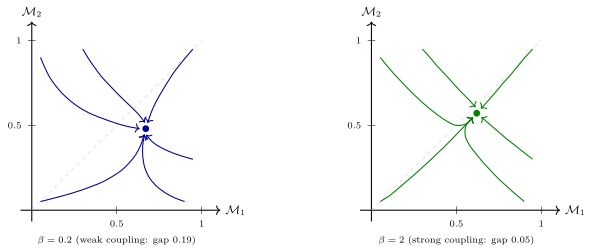
Corollary B.15.6 (Polarization corollary). A heterogeneous population whose growth rates take two values settles into two clusters, one higher and one lower, at every coupling strength: when every \(\alpha_i\sin(2\theta_i) > \gamma_i\) and \(\beta > 0\), the mean-field system is cooperative (each agent’s rate rises with the others’ lucidity) and each \(F_i(M)/M\) is strictly decreasing, so it has a unique positive equilibrium that attracts every nonzero state (a standard result for cooperative systems with concave nonlinearities2). At that equilibrium the gap between two agents satisfies \(F_i(\mathcal{M}_i) - F_j(\mathcal{M}_j) = \beta(\mathcal{M}_i - \mathcal{M}_j)\), so it is inherited from the parameter differences and shrinks like \(1/\beta\) as coupling grows; nothing happens at \(\beta^*\). In the two-agent example of Figure 83 the gap is \(0.30\), \(0.19\), \(0.11\), \(0.05\), \(0.02\) at \(\beta = 0\), \(0.2\), \(0.7\), \(2\), \(5\). This is the model’s mathematical picture of political polarization: where people’s own parameters differ, weak institutions leave the difference standing, and stronger coupling narrows it continuously without closing it.
The Practitioner Effect.
Theorem B.15.7 (Practitioner Theorem). Consider \(n-1\) ordinary agents plus \(1\) practitioner, an agent who maintains a fixed high lucidity \(\mathcal{M}_c\) through sustained practice (§VIII.4). If \(\mathcal{M}_c > \mathcal{M}^*_0\), the practitioner raises the common equilibrium \(\tilde{M}^*\) of the remaining ordinary agents, to first order, by:
\[\begin{equation} \label{eq:b16-practitioner-shift} \Delta\tilde{M} = \tilde{M}^* - \mathcal{M}^*_0 = \frac{\beta(\mathcal{M}_c - \mathcal{M}^*_0)}{n\beta^* + \beta} \end{equation}\]
where \(\mathcal{M}^*_0 = K(\theta)\bigl(1 - \gamma/(\alpha\sin(2\theta))\bigr)\) is the equilibrium without the practitioner, and \(\beta^* = \alpha\sin(2\theta) - \gamma\) here plays the role of the relaxation rate \(-f'(\mathcal{M}^*_0)\).
Derivation. The practitioner contributes an additional pull term \(\frac{\beta(\mathcal{M}_c - \tilde{M})}{n}\) to the mean field, where \(\tilde{M}\) is the mean of the ordinary agents, so the equilibrium condition is \(f(\tilde{M}^*) + \frac{\beta}{n}(\mathcal{M}_c - \tilde{M}^*) = 0\). Linearizing \(f\) around \(\mathcal{M}^*_0\) with \(f'(\mathcal{M}^*_0) = -\beta^*\) gives \(-\beta^*\Delta\tilde{M} + \frac{\beta}{n}(\mathcal{M}_c - \mathcal{M}^*_0 - \Delta\tilde{M}) = 0\), which solves to the formula above.
Scaling behavior.
These dynamics are illustrated in Figure 84.
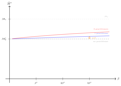
Stability.
Proposition B.15.8 (Linearization and eigenmodes). Perturbing a uniform steady state \(\mathcal{M}_i = \mathcal{M}^*\) of homogeneous agents by \(\varepsilon_i\), the linearized mean-field coupled system yields:
\[\begin{equation} \label{eq:b16-linearized} \frac{d\varepsilon_i}{dt} = \bigl[f'(\mathcal{M}^*) - \beta\bigr]\varepsilon_i + \frac{\beta}{n}\sum_{j=1}^{n}\varepsilon_j \end{equation}\]
At the nonzero equilibrium \(\mathcal{M}^* = \mathcal{M}^*_0\), this system has two classes of eigenmodes:
\[\begin{equation} \label{eq:b16-eigenvalues} \begin{aligned} \nu_1 &= f'(\mathcal{M}^*) = \gamma - \alpha\sin(2\theta) && \text{(uniform mode: $\varepsilon_i = \varepsilon$)} \\ \nu_2 &= f'(\mathcal{M}^*) - \beta = \gamma - \alpha\sin(2\theta) - \beta && \text{(deviation mode: $\sum_i\varepsilon_i = 0$)} \end{aligned} \end{equation}\]
(The eigenvalues are written \(\nu_1, \nu_2\) to avoid clashing with Pattern-awareness \(\lambda(a)\).)
Fixed point classification. Table 24 lists the fixed points of the coupled system, the conditions under which each exists, and its stability.
| Fixed point type | Condition | Stability | Lucidosophy meaning |
|---|---|---|---|
| Uniform high (\(\mathcal{M}^*_0 > \frac{1}{2}\)) | \(\alpha\sin(2\theta) > \gamma + \frac{\alpha}{2}\) | Stable for every \(\beta \geq 0\) | Collective lucidity |
| Uniform low (\(\mathcal{M}^*_0 < \frac{1}{2}\)) | \(\gamma < \alpha\sin(2\theta) < \gamma + \frac{\alpha}{2}\) | Stable for every \(\beta \geq 0\) | Collective semi-obscuration |
| Zero (\(\mathcal{M}_i = 0\)) | Always exists | Unstable if \(\alpha\sin(2\theta) > \gamma\) | Impossible stasis |
| Two-cluster (heterogeneous) | \(\alpha_i\) taking two values, every \(\alpha_i\sin(2\theta_i) > \gamma_i\), any \(\beta \geq 0\) | Unique positive equilibrium; attracts every nonzero state | Political polarization (gap shrinks as \(\beta\) grows) |
Convergence rate. Separate individual relaxation from inter-agent synchronization. By the eigenvalue analysis (Eq. eq:b16-eigenvalues), the deviation mode near the stable equilibrium decays at rate \(\beta + \beta^*\), so:
\[\begin{equation} \label{eq:b16-convergence-rate} \tau_{\text{sync}} = \frac{1}{\beta + \beta^*} \end{equation}\]
Stronger coupling means faster synchronization. Note that under the homogeneous mean-field premise, even at \(\beta = 0\) agents with identical parameters individually relax to the same equilibrium (on the timescale \(1/\beta^*\)), so synchronization still occurs in this degenerate sense; the contribution of coupling is to raise the decay rate from \(\beta^*\) to \(\beta + \beta^*\). For heterogeneous agents with differing parameters, the equilibrium itself keeps a spread at every finite \(\beta\) (shrinking like \(1/\beta\), by the Polarization Corollary), so exact synchronization never occurs; at \(\beta = 0\) each agent settles at its own equilibrium.
Network Topology.
Theorem B.15.9 (Spectral Gap Theorem). The second-smallest eigenvalue \(\mu_2\) of the graph Laplacian (the Fiedler value, or algebraic connectivity) determines the synchronization rate:
\[\begin{equation} \label{eq:b16-spectral-gap} \tau_{\text{sync}}^{\text{network}} = \frac{1}{\mu_2 + \beta^*} \quad \text{(homogeneous agents, near the uniform steady state)} \end{equation}\]
Derivation. Linearizing at the uniform state \(\mathcal{M}^*_0\) with \(f'(\mathcal{M}^*_0) = -\beta^*\) gives \(\dot{\varepsilon} = -(\beta^* I + L)\,\varepsilon\). Because \(L\) is symmetric and positive semidefinite, with eigenvalues \(0 = \mu_1 \leq \mu_2 \leq \cdots \leq \mu_n\) and the constant vector as eigenvector for \(\mu_1\), the deviation modes (orthogonal to the constant vector) decay at the rates \(\beta^* + \mu_k\), \(k \geq 2\), the slowest at \(\beta^* + \mu_2\). \(\square\)
Here \(\beta^* > 0\) is the individual relaxation rate. Larger \(\mu_2\) means faster synchronization. \(\mu_2 = 0\) means the network is disconnected into separate components: agents with identical parameters still relax to the same equilibrium one by one, but subgroups with different parameters settle at their own equilibria, and network-level synchronization is no longer possible.
Topology comparison.
| Network topology | \(\mu_2\) scaling | Sync | Fragmentation resistance | Lucidosophy example |
|---|---|---|---|---|
| Complete graph | \(n\) | Fastest; grows with \(n\) | Strongest (\(n-1\) nodes) | Ideal democracy / commune |
| Small-world | Far above the ring’s; at most about \(d_{\min}\) | Fast for its sparsity | Strong: shortcuts add routes around any removed node | Wisdom traditions / academia |
| Random (Erdős–Rényi) | \(\sim pn\) when \(p \gg (\log n)/n\) | Grows with density | Grows with density | Modern society |
| Scale-free (hub-and-spoke) | At most about \(d_{\min}\) (a star: exactly \(1\)) | Bounded, whatever the size | Weakest: removing the hub splits it | Social media / celebrity networks |
| Ring lattice | \(\sim 4\pi^2/n^2\) | Slowest for large \(n\) | Weak: removing two nodes splits it | Isolated villages |
The five topologies are depicted in Figure 85.
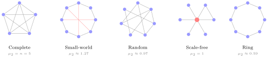
Worked Example
A two-agent example. Return to the simplest case, two agents with identical parameters \(\alpha, \gamma, \theta\) and symmetric coupling \(\beta_{12} = \beta_{21} = \beta\). Suppose \(\mathcal{M}_1 = 0.6\) (a lucid agent) and \(\mathcal{M}_2 = 0.1\) (an obscured agent), with \(\beta = 0.3\). Because the coupled master equation (Assumption B.15.1) normalizes the social term by \(1/n\), the coupling term pushes \(\mathcal{M}_2\) upward by \(\frac{1}{2}\cdot 0.3 \times (0.6 - 0.1) = 0.075\) and pulls \(\mathcal{M}_1\) downward by \(\frac{1}{2}\cdot 0.3 \times (0.1 - 0.6) = -0.075\). The lucid agent “pays a cost” for lifting the obscured one. Symmetric coupling is instantaneously redistributive (the two terms sum to zero); the long-run net effect on the pair is set by the nonlinear individual dynamics. The related coupling level is the \(\beta^*\) of Eq. eq:b16-sync-threshold: above it, every gap between homogeneous agents is guaranteed to shrink, which makes it a sufficient condition for synchronization (Proposition B.15.5).
Interpretation
In everyday terms. Picture an office. Each person’s own habits set the level of lucidity (how clearly they see their situation) at which they would settle alone. Conversation among colleagues plays the model’s coupling: it pulls each person toward the group’s average, so those clearer than average are pulled down a little and those less clear are pulled up a little. Arrangements such as regular meetings and training set how strong this pull is. In this model, a colleague who stays steadily lucid raises the level the whole group settles at, and the larger the group, the more thinly that one person’s effect is spread. When habits differ, closer contact narrows the gaps between people and never closes them; as the pull grows from weak to strong the gaps shrink little by little, with no point where things suddenly flip.
From the single master equation (B.14) to the coupled system (B.15), we have traced the mathematical passage from ethics to politics. Four results emerged, each with no single-agent counterpart:
In these models the passage from “I” to “we” is gradual: coupling does its work continuously, and no single strength of institutions switches a society from fragmented to synchronized.
From ethics to politics. The master equation (B.14) describes the inner life of a single agent. The coupled system (B.15) describes political life. The passage from one to the other, from \(\frac{d\mathcal{M}}{dt}\) to \(\frac{d\mathcal{M}_i}{dt}\) with coupling, is the mathematical form of the passage from ethics (Chapter §VI) to political philosophy (Chapters §X–§XII). The coupling term \(\beta_{ij}(\mathcal{M}_j - \mathcal{M}_i)\) is where politics enters mathematics: it says that my lucidity is never entirely my own affair.
What presence does. The coupling term says: when you are surrounded by people more lucid than you (\(\mathcal{M}_j > \mathcal{M}_i\)), their presence pulls you upward; when surrounded by the less lucid, their influence pulls you downward. This is the mathematical form of the practitioner’s function (§VIII.4): the practitioner raises the group’s \(\beta_{ij}\) values and serves as a high-\(\mathcal{M}\) node. In this model, a lucid presence in a community does more than “set a good example”: it shifts the equilibrium of everyone around it (Theorem B.15.7). The coupling term \(\beta_{ij}(\mathcal{M}_j - \mathcal{M}_i)\) is the formal expression of what every teacher, mentor, and sage has always known: presence itself has an effect.
Institutions supply coupling. In a mean-field regime, the coupling \(\beta\) is supplied by institutional structures (educational systems, media, political institutions). This is why institutional design (§XI.3) is more than a convenience: in this model, institutions set how strongly and how fast agents are pulled toward \(\bar{\mathcal{M}}\), while individual parameters set where \(\bar{\mathcal{M}}\) itself lies. The model is not calibrated to social data, so what it supports is that qualitative judgment, not any quantitative necessary condition.
Reading the contraction level. \(\beta^*\) is a sufficient institutional strength. When institutions (education, media, political structures) provide coupling above it, differences between homogeneous agents shrink at a rate of at least \(\beta - \beta^*\) from any starting point; below it that guarantee lapses, though homogeneous agents still converge.
Institutional time. \(\tau_{\text{sync}}\) is the “institutional time” a collective needs to find consensus. A heterogeneous society with zero coupling has no consensus mechanism: each member stays at its own equilibrium, and coupling narrows that spread without closing it. A strongly coupled society converges rapidly, but this does not automatically mean convergence toward the right place. Individual parameters determine whether the common destination is high lucidity or low lucidity; coupling only determines how quickly agents are pulled together.
Two kinds of mode. \(\nu_1\) governs the overall collective lucidity level (depends only on individual parameters, independent of coupling: identical agents cannot exceed their shared individual ceiling by mutual encouragement alone). \(\nu_2\) governs inter-individual divergence; coupling \(\beta\) makes \(\nu_2\) more negative, accelerating convergence.
The topology of social media. Social media creates a scale-free topology: a few influencers connected to millions, while most people have weak mutual connections. When most people hang off a few hubs and have few ties of their own, \(\mu_2\) stays bounded by that thin minimum degree however large the network grows, so synchronization gains nothing from scale, and removing a few hubs splits the network apart. Ancient wisdom traditions (tightly interconnected small communities, i.e., small-world networks) were topologically better placed in both respects. Once social media is modeled this way, the judgment follows from spectral theory; the modeling step is where it can be contested.
Insights
A group of people with the same habits cannot raise their shared ceiling by encouraging one another; contact only decides how fast they converge. The members of a reading circle all read in much the same way: however often they meet, each still settles at the level they would reach alone, and frequent meetings only bring them there together sooner. In this model this rests on the members sharing the same rates of growth and loss and the same balance, with influence passing between people in proportion to the gap between them; raising the shared level takes changing each person’s own conditions, or adding a practitioner whose lucidity is higher.
When people’s own conditions differ, closer ties shrink the gap between them without ever erasing it, and there is no tipping point along the way. Residents of two neighborhoods learn under different conditions: the more they mix, the closer their levels come, yet the difference in conditions keeps leaving a gap in the outcome. In this model the conclusion requires each person’s own growth to outpace loss, and it describes a group whose growth rates fall into two levels; the model is not calibrated to social data, so it gives the direction and cannot say how large the gap is.
A lone agent cannot restart from zero; in a coupled population with \(\beta > 0\) and a positive mean Lucidity, zero is no longer the end of the road. In B.14 the right-hand side vanishes at \(\mathcal{M} = 0\), making zero an absorbing state (Table 23); in the mean-field Equation (eq:mean-field), the individual term vanishes at \(\mathcal{M}_i = 0\) and the right-hand side reduces to \(\beta\bar{\mathcal{M}}\). In this model exactly one term can move a fully obscured agent off zero: the pull of other people’s Lucidity, carried by the coupling.
To first order, what practitioners achieve depends only on their share \(k/n\) of the population: the same practitioner placed in a group a thousand times larger produces roughly a thousandth of the lift. Extending Equation (eq:b16-practitioner-shift) to \(k\) practitioners gives \(\Delta\tilde{M} \approx \frac{(k/n)\,\beta(\mathcal{M}_c - \mathcal{M}^*_0)}{\beta^* + (k/n)\,\beta}\), in which the head count enters only as a proportion; when \(n\beta^* \gg \beta\), one practitioner’s effect is close to inversely proportional to \(n\). In this model, then, the levers for moving a large population are the share of practitioners and the coupling strength \(\beta\), given \(\mathcal{M}_c > \mathcal{M}^*_0\) and within the first-order approximation of Theorem B.15.7.
How much speed the network structure can add to convergence is capped by its least-connected member. By the Spectral Gap Theorem (Theorem B.15.9), the slowest deviation among homogeneous agents near the uniform state decays at \(\beta^* + \mu_2\), the network’s contribution is \(\mu_2\), and Fiedler’s bound \(\mu_2 \leq \frac{n}{n-1}\,d_{\min}\) looks only at the minimum degree (Table 25). Adding links to a hub leaves that cap where it is, and the hub-and-spoke graph of Figure 85 keeps \(\mu_2 \leq 1\) however many spokes it gains; raising the cap requires giving the least-connected people more ties.
Scope and limits
Linear diffusive coupling is the simplest model. The linear diffusive coupling \(\beta_{ij}(\mathcal{M}_j - \mathcal{M}_i)\) is the simplest model in which influence is proportional to the lucidity gap. Real social influence is far more complex (asymmetric, context-dependent, mediated by power and affect). The model captures the qualitative insight that lucidity is socially contagious; the specific coupling constants \(\beta_{ij}\) are not empirically measurable. The results of this section (synchronization, the practitioner shift, the Fiedler-value rate) are structural consequences of diffusive coupling, not predictions calibrated to social data.
B.16 · Collective Lucidity and Emergence
Question: When does the collective lucidity of a coupled group rise above the individual average, and when does it fall below?
Requires: The coupling setup of B.15.
Yields: The emergence inequality (Proposition B.16.2) and sufficient conditions for collective lucidity to rise above or fall below the individual average (Propositions B.16.3 and B.16.4).
B.15 follows how each agent’s lucidity evolves under coupling. This section asks about the group as a whole: how its lucidity is measured, and when it departs from the members’ average.
Setup
Definition B.16.1 (Collective lucidity function). Define \(\Psi\) as a general functional of individual lucidities and coupling structure:
\[\begin{equation} \label{eq:b16-phi-definition} \Psi(\mathcal{M}_1, \ldots, \mathcal{M}_n;\; W) = \operatorname{clip}_{[0,1]}\!\left( \bar{\mathcal{M}} + \eta\, \frac{\sum_{i < j} w_{ij}\,g(\mathcal{M}_i, \mathcal{M}_j)} {\sum_{i < j}|w_{ij}|} \right) \end{equation}\]
where \(W = \{w_{ij}\}\) is the coupling matrix (which may have negative entries for destructive coupling), \(\eta \in [0,1]\) controls the maximum interaction contribution, and the denominator is replaced by \(1\) if all \(w_{ij}=0\). The clipping keeps \(\Psi\) on the same normalized scale as individual lucidity. The synergy function is \(g(\mathcal{M}_i, \mathcal{M}_j) = \min(\mathcal{M}_i, \mathcal{M}_j) \cdot (1 - |\mathcal{M}_i - \mathcal{M}_j|)\).
Reading. \(g\) captures two intuitions: (1) both agents need positive lucidity for synergy to exist (the \(\min\) factor); (2) the smaller the gap, the greater the synergy (the \((1 - |\mathcal{M}_i - \mathcal{M}_j|)\) factor). Under perfect synchronization (\(\mathcal{M}_i = \mathcal{M}_j\)), \(g = \mathcal{M}_i\); under complete fragmentation (one at 0, the other at 1), \(g = 0\). The sign and magnitude of \(w_{ij}\) determine whether coupling enhances or degrades collective lucidity.
Write the normalized synergy as \[S_W = \frac{\sum_{i < j} w_{ij}\,g(\mathcal{M}_i,\mathcal{M}_j)}{\sum_{i < j}|w_{ij}|},\] so that \(\Psi\) before clipping is \(\bar{\mathcal{M}} + \eta S_W\). The emergence inequality and the superadditivity and sub-additivity propositions below all use this quantity.
Results and Proofs
Proposition B.16.2 (Emergence inequality). In the spirit of the Emergence Theorem (T2), the model lets collective lucidity differ from the aggregate of individual lucidities; the difference is built into the functional \(\Psi\) of Definition B.16.1, and it follows from that definition, not from T2. Under \(\Psi\), collective lucidity departs from the individual mean whenever the normalized synergy \(S_W\) of the setup is non-zero, \(\eta > 0\), and the result stays inside \([0,1]\):
\[\begin{equation} \label{eq:emergence-inequality} \mathcal{M}_{\text{collective}} \neq \frac{1}{n}\sum_{i=1}^{n} \mathcal{M}_i \qquad\text{(when $\eta S_W \neq 0$ and $\Psi$ is not clipped)} \end{equation}\]
The collective lucidity function \(\Psi\) depends on the coupling structure:
\[\begin{equation} \label{eq:collective-phi} \mathcal{M}_{\text{collective}} = \Psi\bigl(\mathcal{M}_1, \ldots, \mathcal{M}_n;\; \{\beta_{ij}\}\bigr) \end{equation}\]
For a group of individually lucid agents with zero coupling (\(\beta_{ij} = 0\)), collective lucidity is nothing but the individual mean: nothing emerges between them. A group whose coupling is constructive, so that the weighted synergy is positive, can achieve collective lucidity exceeding the individual average; this is the mathematical form of democracy’s added value (§XI.6). In the functional \(\Psi\), what counts is the sign pattern and the relative weights of the coupling: multiplying every coupling weight by the same positive number leaves \(\Psi\) unchanged.
The emergence inequality (Eq. eq:emergence-inequality) says collective lucidity departs from the individual mean. But it does not tell us when collective lucidity is greater than the mean and when it is less, nor does it address the boundary case where zero net synergy leaves the two equal. The next two propositions give sufficient conditions for both directions under the normalized functional of Definition B.16.1.
Proposition B.16.3 (Superadditivity condition). When coupling is constructive (\(w_{ij} \geq 0\) for all pairs), a sufficient non-saturated condition for collective lucidity to exceed the mean is:
\[\begin{equation} \label{eq:b16-superadditivity} \Psi > \bar{\mathcal{M}} \;\Leftarrow\; S_W > 0 \;\text{and}\; \eta > 0 \;\text{and}\; \bar{\mathcal{M}} + \eta S_W < 1 \end{equation}\]
In words: when constructive coupling generates positive normalized synergy and the result is not already saturated at the upper bound, collective lucidity exceeds the individual mean. This is the quantitative form of the Emergence Theorem (T2) in the lucidity domain: constructive coupling creates emergence.
Proposition B.16.4 (Sub-additivity condition, emergent obscuration). When coupling is destructive (\(w_{ij} < 0\), modeling manipulative or asymmetric influence):
\[\begin{equation} \label{eq:b16-anti-superadditivity} \Psi < \bar{\mathcal{M}} \;\Leftarrow\; S_W < 0 \;\text{and}\; \eta > 0 \;\text{and}\; \bar{\mathcal{M}} + \eta S_W > 0 \end{equation}\]
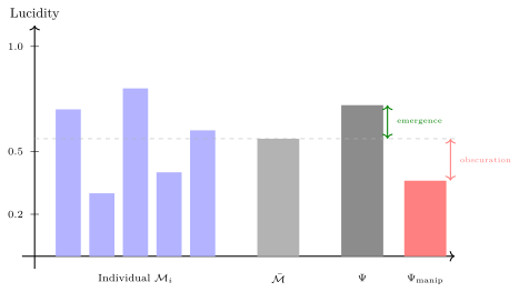
Interpretation
In everyday terms. Picture a project meeting. The model starts from the average lucidity of the members (how clearly each sees the situation), then adds or subtracts an amount for each relationship between two members. Two colleagues who build on each other’s points form a constructive link, which adds to the group’s score; someone who steers the discussion by pressure or misleading claims forms a destructive link, which subtracts. How much a link adds or subtracts also depends on the two people in it: when both are lucid and close to each other in level, the link carries the most weight. In this model, then, the group can end up clearer than its members’ average, or more confused, while no member has changed at all; only the structure of their relationships has.
Propaganda and emergent obscuration. The sub-additivity condition (Proposition B.16.4) formalizes the mathematical structure of propaganda: a low-lucidity node exerting asymmetric destructive influence (\(w_{\text{propagandist}\to\text{public}} < 0\)) lowers collective lucidity below the individual mean. The group becomes less lucid than its members’ average: the individuals have not changed; the coupling structure manufactured systematic obscuration (Figure 86). Algorithmically optimized misinformation, sycophantic AI feedback, and attention-hijacking platforms are all mechanisms that produce negative \(w_{ij}\).
Insights
Bring lucid people together without any interaction between them, and the group’s lucidity is simply their average; nothing extra appears. A company hires several capable experts from different places, and each works alone without exchanging ideas; in this model the group’s lucidity equals exactly the average of theirs. For the group to rise above its average, the members’ interactions must be constructive on balance, the model must give interaction some weight, and the group’s lucidity must not already sit at the top of the scale.
When a group acts more confused than its members’ average, the cause can lie entirely in the relationships, with no member having become any less lucid. In a neighborhood where everyone carries on as before, one person keeps spreading misleading claims and stirring mutual suspicion, and the neighborhood’s judgment as a whole drops below its residents’ average. In this model this requires the relationships, weighed by their strength, to be destructive on balance, interaction to carry some weight in the model, and the result not to have hit the bottom of the scale already; in such a case, what needs examining is who influences whom, and how.
With individual Lucidities fixed, collective Lucidity reads the pattern of interaction and ignores its volume: multiply every coupling weight by the same positive number and \(\Psi\) stays the same. In Equation (eq:b16-phi-definition) numerator and denominator are both linear in the weights, so the scale factor cancels. In B.15 the strength of coupling sets how fast members converge; in \(\Psi\) only the signs of the couplings and their weights relative to one another count. In this model, more meetings and denser messaging change collective Lucidity only insofar as they change that pattern.
Under this section’s definition, the synergy a pair can contribute is capped by the weaker member’s Lucidity and shrinks as their gap widens, so raising a group’s synergy starts with its weakest members and its widest gaps. The synergy function \(g = \min(\mathcal{M}_i, \mathcal{M}_j)\,(1 - |\mathcal{M}_i - \mathcal{M}_j|)\) is a modeling choice of Definition B.16.1: the pair \((0.9, 0.2)\) has mean Lucidity \(0.55\) and synergy \(0.06\), while the pair \((0.5, 0.5)\) has mean \(0.5\) and synergy \(0.5\). Under this definition, adding one exceptionally lucid member still leaves each of that member’s pairings capped by the other person’s Lucidity.
Destructive coupling does the most damage between two members who are both lucid and close to each other, and one heavy enough negative link can outweigh many positive ones. Each link contributes \(w_{ij}\,g(\mathcal{M}_i, \mathcal{M}_j)\) to \(S_W\), and \(g\) is largest when both members are lucid and close, so a negative weight of a given size removes the most synergy there. Propositions B.16.3 and B.16.4 turn on the sign of the weighted sum \(S_W\) (together with \(\eta > 0\) and no clipping), and the number of positive or negative links never enters: in this model a group whose relationships are overwhelmingly constructive can still fall below its members’ average.
B.17 · Cosmological Limits: Civilizational Silence and the Dark Forest
Question: What follows when lucidity dynamics is carried to the scale of civilizations and the cosmos, and which further assumptions does it take?
Requires: The gradient of B.12; the coupling of B.15; the game theory of B.11; derivatives.
Yields: A detectability model and the conditional criterion for T6 (Proposition B.17.4), the Dark Forest Theorem (Theorem B.17.5), and the Trust Threshold Theorem (Theorem B.17.6).
This section provides the mathematical formalization for Chapters §XV (Civilizational Lucidity) and §XVI (The Dark Universe and Dual Silence). For the philosophical argument and case analysis, see §XV and §XVI.
B.15 built the mathematical framework for multi-agent lucidity. This section extends the scale from human society to interstellar civilizations.
Setup
The setup of this section has three parts: the detectability model, the light-cone form of coupling between civilizations, and the detection risk of broadcasting.
Let a civilization’s detectability \(D\) be proportional to its Pattern-domain activity, and lucidity be \(\mathcal{M} = \lambda \cdot \xi\). When a civilization evolves along the gradient \(\nabla\mathcal{M} = (\xi, \lambda)\) with \(\lambda \gg \xi\), the gradient favours \(\xi\), the Mystery domain: both components are positive, and the \(\xi\)-component is the larger.
Assumption B.17.1 (Detectability). Let a civilization’s detectability at time \(t\) be:
\[\begin{equation} \label{eq:b17-detectability} D(t) = \lambda(t) \cdot E(t) \end{equation}\]
where \(E(t)\) is energy output (the Kardashev scale3 \(\propto\) degree of Pattern-domain exploitation). Meanwhile, lucidity is \(\mathcal{M}(t) = \lambda(t) \cdot \xi(t)\), subject to the constraint \(\lambda + \xi + \delta = 1\) (the model stipulates \(\delta > 0\), in the spirit of Postulate 6).
Assumption B.17.2 (Light-cone coupling). The coupling strength between civilizations must respect the causal structure of spacetime, which fixes the indicator factor below; the exponential decay with distance, and its scale \(c\tau\), are a modeling choice. We formalize this as:
\[\begin{equation} \label{eq:b18-light-cone} \beta_{ij}(t) = \beta_0 \cdot e^{-d_{ij}/(c \cdot \tau)} \cdot \mathbf{1}_{[t > d_{ij}/c]} \end{equation}\]
where \(\beta_0\) is the baseline coupling strength (depending on communication technology level), \(d_{ij}\) is the distance between civilizations \(i\) and \(j\), \(c\) is the speed of light, \(\tau\) is the civilization’s characteristic timescale (e.g., technology development cycle), and \(\mathbf{1}_{[\cdot]}\) is the indicator function.4 The coupling is zero before the light travel time has elapsed (causality), and decays exponentially with distance thereafter. At interstellar distances, civilizations are effectively decoupled.
Definition B.17.3 (Detection risk function). Each civilization faces a risk–reward calculus when choosing its detectability level:
\[\begin{equation} \label{eq:b18-detection-risk} R_i(D_i) = p_{\text{detect}}(D_i) \cdot p_{\text{hostile}}(\xi_j = 0) \cdot \ell_i \end{equation}\]
where \(p_{\text{detect}}(D_i)\) is the probability that civilization \(i\) is detected (monotonically increasing in \(D_i\)), \(p_{\text{hostile}}(\xi_j = 0)\) is the probability that a detecting civilization \(j\) is hostile (which depends directly on the prior probability that \(\xi_j = 0\)), and \(\ell_i\) is the loss from a hostile strike. The key insight: \(p_{\text{hostile}}\) depends on assumptions about \(\xi_j\). The model takes as premises that \(p_{\text{hostile}} \to 1\) under Dark Forest assumptions (\(\xi_j \to 0\) for all \(j\)) and that \(p_{\text{hostile}} < 1\) under lucidity assumptions (\(\xi_j > 0\) possible).
Results and Proofs
Civilizational Silence.
If a civilization evolves along the lucidity gradient (i.e., chooses to maximize \(\mathcal{M}\) rather than \(D\)), then:
When \(\lambda > \xi\), \(\nabla\mathcal{M} = (\xi, \lambda)\) raises both components and raises \(\xi\) faster: the civilization invests more in the Mystery domain
Along this gradient \(\dot{\lambda} = \xi > 0\), so a stable \(E(t)\) leaves \(D(t)\) rising; the growth of \(D(t)\) reverses only if \(E(t)\) declines at a relative rate faster than \(\xi/\lambda\)
Detectability decreases only under this additional energy-response assumption
Proposition B.17.4 (Conditional criterion for T6, the Civilizational Silence Theorem). Let a civilization evolve along \(\nabla\mathcal{M}\). Since \(D(t)=\lambda(t)E(t)\), \[\begin{equation} \label{eq:b17-detectability-derivative} \frac{dD}{dt} = D(t)\left(\frac{\dot{\lambda}(t)}{\lambda(t)} + \frac{\dot{E}(t)}{E(t)}\right). \end{equation}\] Therefore, if there exists a time \(t^*\) such that for all \(t > t^*\): \[\begin{equation} \label{eq:b17-silence} \frac{\dot{E}(t)}{E(t)} < -\frac{\dot{\lambda}(t)}{\lambda(t)}, \end{equation}\] then \(\frac{dD}{dt} < 0\), and the civilization becomes progressively quieter after \(t^*\).
Along the unconstrained gradient of B.12, \(\dot{\lambda} = \xi\), so the condition reads \(\dot{E}/E < -\xi/\lambda\). The window \(\lambda > \xi\) stated in T6 does not appear in this inequality; it enters through the theorem’s maturity-choice premise, since only while \(\lambda > \xi\) does the gradient favour mystery-awareness.
For the classification of civilizational fates, contemporary case analysis, and the philosophical discussion, see §XV.
The Dark Forest.
For the philosophical discussion of the Dark Forest theory, its axioms, and the Chain of Suspicion, see §XVI.
Three-Body \(\to\) Lucidosophy mapping.
| Three-Body Concept | Lucidosophy Interpretation | Formal Expression |
|---|---|---|
Three-Body Concept |
Lucidosophy Interpretation | Formal Expression |
Dark Forest Theory |
\(\xi \to 0\) limit: Mystery-awareness vanishing | \(\mathcal{M}_i \to 0\;\forall i\) |
| Cosmic Sociology Axiom 1 (Survival) | Pure Pattern-domain axiom | \(\max \lambda_i\) s.t. \(\delta_i > 0\) |
| Cosmic Sociology Axiom 2 (Expansion) | \(\lambda\)-maximization under scarcity | \(d\lambda/dt > 0\) |
| Chain of Suspicion | \(\beta = 0\), assume \(\xi_j = 0\) | Trust impossible |
| Wallfacer Project5 | P17 at existential scale | Cognitive sovereignty |
| Sophon6 | P19 at cosmic scale | Destroying target’s cognitive ecology |
| Dimension Reduction Attack7 | Forcing \(\delta \to 1\) | Cosmic obscuration attack |
Theorem B.17.5 (T7, Dark Forest Theorem). In the multi-agent setting of B.15 with \(n\) civilizations, suppose:
\(\beta_{ij} = 0\) for all \(i \neq j\) (no communication),
\(\xi_i \to 0\) for all \(i\) (vanishing Mystery-awareness; the Dark Forest is this limit, since \(\xi = 0\) itself lies outside the range T1 allows),
each civilization maximizes \(\lambda_i\) subject to survival,
whatever the other civilizations do, broadcast exposure creates expected strike loss greater than any broadcast benefit,
whatever the other civilizations do, armament cost is lower than the expected loss from accidental detection while unarmed.
Then universal silence with preemptive strike preparation is the unique pure-strategy Nash equilibrium of the simplified broadcast and armament game, in which each civilization chooses to broadcast or stay silent and to arm or not: \[\begin{equation} \label{eq:b18-dark-forest} \sigma_i^* = (\text{silent},\;\text{armed}) \quad \forall\, i \end{equation}\]
For the philosophical argument, see T7.
By hypothesis 4, read for every profile of the others’ actions, broadcasting (\(D > 0\)) has lower expected payoff than silence (\(D = 0\)), so silence strictly dominates broadcasting. By hypothesis 5, read the same way, armament strictly dominates non-armament. A profile in which some civilization plays a strictly dominated action is no equilibrium, and the profile in which every civilization plays its dominant actions is one; therefore \((\text{silent}, \text{armed})\) is the unique pure-strategy Nash equilibrium. The derivation uses hypotheses 4 and 5 only. Hypotheses 1 to 3 describe the setting that makes those payoffs plausible: as \(\xi \to 0\), every civilization sinks into the Pattern Trap (§XV.3), and capability (\(\lambda\)) revealed by detection can only be read as threat, since inferring benevolence would take \(\xi > 0\); with \(\beta = 0\) no channel can revise that reading. They take no part in the dominance step. The conclusion is conditional on the payoff assumptions, which is why this is graded as a demonstration rather than a proof.
Subsumption result. The Dark Forest is a limit of the framework:
\[\begin{equation} \label{eq:b18-subsumption} \text{Dark Forest Theory} = \text{Lucidity Framework}\big|_{\xi \to 0,\; \beta = 0,\; \text{survival payoffs}} \end{equation}\]
The Dark Forest holds within its domain, but it is incomplete. It is the limit of the lucidity framework as Mystery-awareness goes to zero, with communication nil and the survival payoffs holding. The restriction is interpretive: because the demonstration of T7 runs on the payoff assumptions, what the bar records is the setting in which those payoffs become plausible. For the philosophical interpretation, see §XVI.
The Cosmic Game.
Cosmic payoff matrix. Simplifying to the two-player case reveals the game-theoretic structure:
| Civ B: Broadcast | Civ B: Silent | |
|---|---|---|
| Civ A: Broadcast | If \(\xi > 0\): cooperation possible If \(\xi = 0\): mutual annihilation |
A exposed, B hidden |
| Civ A: Silent | B exposed, A hidden | No interaction |
Analysis. Under Dark Forest assumptions (\(\xi \to 0\)) plus the strong payoff assumptions in T7, (Silent, Silent) is the unique pure-strategy equilibrium in the broadcast/silent game. Under lucidity assumptions (\(\xi > 0\)), the displayed two-strategy matrix is no longer sufficient to decide dominance, because a civilization can be silent in the broadcast sense while actively listening. A fuller three-action model would distinguish Broadcast, Low-detectability Listen, and Full Silence. The expanded model is not written out here; the expectation is that in it, low-detectability listening becomes weakly preferable for sufficiently high \(\xi\) and sufficiently low detection risk. The selection between equilibria depends on \(\xi\), the dimension that the Dark Forest theory excludes by construction.
Theorem B.17.6 (T8, Trust Threshold Theorem). In one stylized threshold model, let two civilizations \(i, j\) have coupling strength \(\beta_{ij}\), dissipation rates \(\gamma_i, \gamma_j\) with \(\gamma_{\max} = \max(\gamma_i, \gamma_j)\), and Mystery-awareness \(\xi_i, \xi_j > 0\) respectively. If the coupling strength exceeds the trust threshold \[\begin{equation} \label{eq:b18-trust-threshold} \beta_{ij} > \beta_{ij}^{\dagger} = \frac{\gamma_{\max}}{\min(\xi_i, \xi_j)}, \end{equation}\] then cooperation is an equilibrium of this model. The model’s own criterion is \(\beta_{ij}\xi_j > \gamma_i\) and \(\beta_{ij}\xi_i > \gamma_j\), that is, \(\beta_{ij} > \max(\gamma_i/\xi_j,\, \gamma_j/\xi_i)\), a bound that never exceeds \(\beta_{ij}^{\dagger}\); when the two dissipation rates are equal the two bounds coincide, and the condition is then necessary as well as sufficient. As \(\min(\xi_i, \xi_j) \to 0\), both bounds diverge: infinite coupling is required, which is the Chain of Suspicion.
For the philosophical argument, see T8.
The model posits, as a modeling choice of its own (the coupling of B.15 acts on lucidity gaps and contains no such term), that civilization \(i\) gains \(\beta_{ij} \cdot \xi_j\) from civilization \(j\) (coupling strength times the other’s Mystery-awareness: only a civilization that perceives the other’s inner life can ground trust); symmetrically, \(j\) gains \(\beta_{ij} \cdot \xi_i\) from \(i\). Cooperation is an equilibrium when each side’s gain exceeds its own dissipation: \(\beta_{ij}\xi_j > \gamma_i\) and \(\beta_{ij}\xi_i > \gamma_j\). Since \(\gamma_i, \gamma_j \leq \gamma_{\max}\) and \(\xi_i, \xi_j \geq \min(\xi_i, \xi_j)\), the single condition \(\beta_{ij} \cdot \min(\xi_i, \xi_j) > \gamma_{\max}\) implies both, and \(\max(\gamma_i/\xi_j, \gamma_j/\xi_i) \leq \gamma_{\max}/\min(\xi_i, \xi_j)\). With \(\gamma_i = \gamma_j = \gamma\), the criterion reads \(\beta_{ij} > \gamma/\min(\xi_i, \xi_j) = \beta_{ij}^{\dagger}\) exactly. This exemplary functional form serves the qualitative theorem in the main text and is not a unique law of cosmic politics, which is why this is graded as a demonstration rather than a proof.
This threshold model reveals the mathematical essence of the Chain of Suspicion: it is inevitable only under the specific premise that Mystery-awareness vanishes. Once \(\xi > 0\), finite communication can break the Chain of Suspicion; it suffices, for instance, that coupling times the weaker party’s Mystery-awareness exceed the larger dissipation rate: the thinner the channel, the more Mystery-awareness it takes. In this model, a civilization that perceives the inner life of the other deeply enough can build trust even with weak communication, while a civilization with zero Mystery-awareness cannot trust even with perfect communication.
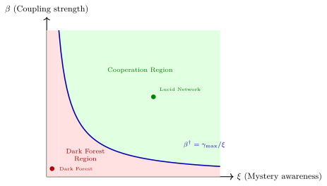
Interpretation
In everyday terms. Picture two great powers that distrust each other: each can see the other’s strength, and neither can see the other’s intentions. If both assume the other only calculates, and both assume that being exposed always costs more than it gains, then hiding and arming is each side’s safest choice; this is the Dark Forest in the model. Mystery-awareness (the capacity to sense what lies beyond one’s grasp, including another’s inner life) plays the ability to read the other’s intentions, and a hotline and regular contact play coupling. In this model, as long as each side can read the other somewhat and contact is frequent enough, what each side gains from cooperating exceeds its own losses, and cooperation holds. The weaker reader sets the bar: the shallower its reading, the more contact it takes.
Pareto analysis. In the extended game that admits \(\xi > 0\), if cooperation yields each side a net lucidity gain, as the threshold model assumes above its threshold (mutual lucidity enhancement, as in B.16’s superadditivity analysis), both civilizations do better cooperating, and the Dark Forest’s (Silent, Silent) equilibrium is Nash but not Pareto optimal. The tragedy of the Dark Forest is a coordination failure. This structurally parallels B.16’s anti-superadditivity result (asymmetric coupling causing collective lucidity to fall below the individual average): in both cases, the failure lies in the interaction structure, and the interaction structure is shaped by \(\xi\) (Figure 87).
Insights
An outcome both sides can hold may be one both would trade away: silence against silence is stable, while cooperation would leave each side better off. Two companies in the same industry each hold safety data the other could use, and each fears the other will exploit it if it shares first, so neither shares and the standoff stays. In this model this rests on two premises: each side can read the other at least somewhat, and cooperation brings each side a net gain; the standoff then comes from a failure to coordinate, with neither side willing to move first.
When messages travel more slowly than either side changes, the channel is close to no channel at all. Two companies negotiate by letter, and each reply arrives after the other side has already replaced its management, so the letter answers a counterpart that no longer exists. In this model, interstellar civilizations have almost no contact with one another for this reason; the conclusion rests on the premise that a civilization’s own timescale of change is short compared with the time light takes to cross the distance between them, and the exact way contact fades with distance is a modeling choice. If the timescale of change were comparable to the light-travel time, that contact would no longer be negligible.
In this model a civilization following the Lucidity gradient still grows its Pattern-awareness; to grow quieter it needs a further choice, letting energy output fall in relative terms faster than Pattern-awareness rises. Along the gradient of B.12, \(\dot{\lambda} = \xi > 0\), so with energy output held level the detectability \(D\) still rises; Proposition B.17.4 requires Equation (eq:b17-silence), that is, \(\dot{E}/E < -\xi/\lambda\). Reading T6, then, “turning toward Mystery” and “reining in energy” are two separate premises, and civilizational silence follows only when both hold.
The Dark Forest conclusion rests entirely on two payoff assumptions; in this stylized game, leaving the Dark Forest requires one of them to fail. The argument for T7 uses only condition 4 (for every combination of the others’ actions, the expected loss from broadcasting exceeds its gain) and condition 5 (arming strictly dominates); \(\xi \to 0\) and \(\beta = 0\) describe the setting that makes those payoffs plausible. Table 27 shows that once \(\xi > 0\) is admitted, cooperation becomes possible in the (Broadcast, Broadcast) cell, so condition 4’s “for every combination” can no longer be taken for granted; the extended three-action model is not written out here, so this step remains an expectation.
In the threshold model the weaker side sets the price of trust: halve the weaker side’s Mystery-awareness and the required communication strength doubles; let it approach zero and no finite communication suffices. Equation (eq:b18-trust-threshold) gives \[\beta_{ij}^{\dagger} = \frac{\gamma_{\max}}{\min(\xi_i, \xi_j)},\] with the larger dissipation rate on top and the smaller Mystery-awareness below, so one side’s depth cannot make up for the other’s shallowness. The model is illustrative (taking the gain as \(\beta_{ij}\xi_j\) is a modeling choice), and the threshold is a sufficient condition for cooperation to be an equilibrium, exact as a boundary only when the two dissipation rates are equal (Theorem B.17.6).
Scope and limits
What the appendix supplies. Appendix B supplies the mathematical condition that the philosophical argument in T6 must satisfy; \(\nabla\mathcal{M}\) alone does not yield civilizational silence.
Part V · From Mathematics to Practice
How do mathematical structures translate into embodied daily practice? This part distills the abstract insights of the preceding four parts into awareness exercises, self-assessment scales, and action guides.
This part is the single section B.18, which draws on B.2 to B.16.
B.18 · From Mathematics to Practice
Question: How does the preceding mathematics become daily practice?
Requires: The matching sections among B.2 to B.16.
Yields: Awareness exercises, a directional self-assessment scale for obscuration, and an action guide.
Behind an equation lies a way of seeing the world, and it can be translated into concrete daily practice. This section distills the mathematical insights of B.2–B.16 into three types of practical tools: awareness exercises, self-assessment scales, and action guides. These tools complement §VIII (Practice): that chapter starts from lived experience, this section starts from mathematical structure, and both point in the same direction: living more lucidly.
B.18.1 · Awareness Exercises: Seeing Daily Life Through Mathematical Eyes
The exercises below borrow the model’s quantities as analogies: entropy, gradients and feedback coefficients cannot be measured in daily life, and the exercises borrow only the shape of these structures.
Entropy and Finitude (B.2 + B.8).
Energy audit. Each week, review your “energy inputs” (sleep, nutrition, exercise, nourishing relationships) against your “entropy-increasing drains” (stress, overwork, harmful habits). Your life is a dissipative structure (it holds \(S_{\text{organism}}\) low only by exporting entropy) that requires continuous negative-entropy input to maintain. When drains exceed inputs, you are accelerating your own thermodynamic conclusion.
The \(r(t,T)\) exercise. Choose an ordinary moment (drinking a glass of water, walking a stretch of road) and remind yourself: because your life is finite and so is its total \(V(T)\), the weight \(r(t,T)\) here is positive, and the stretch of time around this moment makes a positive contribution to your total experience.
Gradients and Curiosity (B.3).
Curiosity gradient check. When life feels dull, ask yourself: in which domains has my \(D_{\text{KL}}\) approached zero? Where are there unexplored non-uniformities I know nothing about? List three fields you are completely ignorant of; there lie unconsumed gradients, fuel for curiosity.
Gradient dissipation awareness. In your most familiar domain, notice that “successfully exploiting a gradient is destroying it”: the more successful you are, the weaker the driving force. This is the structure B.3 characterizes. Treat it as a signal: time to seek new gradients.
Selection and Belief (B.4).
Belief update journal. Once a month, record: what new evidence changed my beliefs this month? If the answer is “nothing,” you may be in the obscured state \(P(H \mid E) \approx P(H)\). Bayes’ theorem says: no updating means no learning.
Over-selection self-check. Examine your information sources: do your news, podcasts, and social media all point in the same direction? If so, your belief distribution \(P_n\) is collapsing onto a single point \(x^*\), and diversity is being destroyed by selection. The remedy is simple: deliberately subscribe to one source you disagree with.
Feedback and Obscuration (B.5 + B.6).
Feedback coefficient estimation. For your strongest belief, estimate whether its effective feedback coefficient \(\alpha + \beta \cdot R'(b)\) exceeds 1. The symptom: the more you believe X, the more the algorithm pushes X-supporting content, the more you believe X. An active loop tells you only that the recommendation term is positive. Deepening alone does not show that 1 has been crossed: below 1 a belief can still rise steadily toward a fixed level. The test for crossing 1 is whether, with no new evidence, the belief keeps growing without settling at any level.
The \(\gamma\)-injection exercise. Spend thirty minutes each week deliberately “injecting negative feedback”: read an author you disagree with, converse with someone of a different opinion, scrutinize your most certain judgment. This is increasing \(\gamma \cdot C(b_t)\) in Equation (eq:lucidity-feedback).
Emergence and Wholes (B.10).
Emergence awareness. Observe a complex system (a flock of birds, the flow of a conversation, a team project’s outcome) and notice the emergent pattern of the whole. This pattern exists in none of the individual parts. Remind yourself that here \(\mathcal{I}_{\text{em}}\) may well be positive; understanding the parts does not equal understanding the whole.
Creating conditions for emergence. Emergence requires three conditions: diversity (engage with people of different backgrounds), connection (build deep relationships that allow genuine interaction), and time (give processes patience; emergence needs iterated interaction).
Cognitive Limits (B.9).
The “I don’t know” exercise. Each day, find one question you genuinely do not know the answer to, and sit with that not-knowing. Do not rush to seek an answer. Gödel tells us: some undecidability is structural, not temporary. Making peace with uncertainty is itself a capability.
Framework audit. Once a month, examine your most frequently used “explanatory frameworks” (political positions, religious beliefs, theoretical preferences). T3 says: every framework has boundaries. What does your framework obscure? What can it not explain? Can you identify its Gödel sentence, that question it can neither prove nor refute? The “Gödel sentence” here is an analogy: an everyday explanatory framework is no formal system.
The Lucidity Product and Balance (B.12 + B.13).
The weaker-side check. In the area where you invest most, ask which is lower: your Pattern-awareness \(\lambda\) or your Mystery-awareness \(\xi\). Lucidity is their product, and the gradient \(\nabla\mathcal{M} = (\xi, \lambda)\) says that a step on the lower component buys more lucidity. Give part of next month to the weaker side.
Growth and Dissipation (B.14).
The upkeep ledger. In the master equation, lucidity rises through the growth term and drains away at the rate \(\gamma\mathcal{M}\); a nonzero equilibrium exists only when growth outweighs dissipation (\(\alpha\sin 2\theta > \gamma\)). Recall a practice you have stopped: what has been slowly ebbing since? That is the dissipation term as it shows up in daily life.
Coupling and Presence (B.15 + B.16).
The coupling list. List the five people or information sources you deal with most each week. The coupled master equation says your lucidity is pulled toward the lucidity of those you are connected to. Ask whether this list is pulling you up or down.
Noticing negative coupling. Notice an occasion that left a group less lucid than its members’ average: a discussion steered off course, a platform that rewards only agreement. The sub-additivity condition (Proposition B.16.4) says collective lucidity can fall below the individual mean; then the way people are connected is what deserves changing, and no single member need be at fault.
B.18.2 · Obscuration Self-Assessment: A Directional Scale
Based on B.6’s information-theoretic model, the following scale determines direction: is your \(\mathcal{O}_t\) rising or falling? The absolute obscuration degree cannot be calculated.
Information diversity dimension (corresponding to \(I_{\text{new}}(t)\)): In the past month, how many mutually contradictory viewpoints have you encountered? Has your social media feed narrowed or broadened in the past six months? When was the last time you had a deep conversation with someone of a completely different background?
Belief update dimension (corresponding to \(P(H \mid E)\) vs \(P(H)\)): In the past year, how many important beliefs have you changed? Can you clearly state what evidence would make you change your currently strongest belief? Do you hold any “unquestionable” beliefs? If so, that is the state \(P(H) = 1\), where Bayesian updating ceases to function.
Feedback structure dimension (corresponding to \(\alpha + \beta \cdot R'(b)\)): How many negative feedback mechanisms exist in your information environment (friends who disagree, media with opposing views)? Have you actively sought out opinions opposing yours in the past month? Has algorithmic recommendation formed a closed loop: is the content you see increasingly “like you”?
Assessment method: Watch the direction; there is no score or ranking. Are the above indicators improving or deteriorating? The direction of \(\Delta\mathcal{O}_t\) matters more than the absolute value of \(\mathcal{O}_t\).
B.18.3 · Action Guide: From Game Theory to Ethical Decision-Making
Based on B.11’s game-theoretic framework, the following tools help you make more lucid choices when facing ethical dilemmas.
Decision payoff matrix exercise. When facing a difficult choice, draw a simplified \(2 \times 2\) matrix: what are the short-term and long-term payoffs of choosing “lucid action” vs “obscured avoidance”? The exercise makes the implicit incentive structure visible; the numbers need not be precise.
Trust first-mover exercise. This week, show genuine vulnerability to one person. Equation (eq:trust-game) tells you: the first mover in a trust game bears risk, but in a relationship with no fixed last round, where the future weighs enough (\(\rho \geq 1/\chi\) in B.11), the first mover establishes the possibility of reciprocity.
Breaking the obscuration equilibrium. If you detect “collective obscuration” in a group (everyone avoiding the truth, maintaining surface harmony), consider being the first to speak. Equation (eq:collective-lucidity) tells you: while \(p\) is below \(p^*\), each additional person who speaks brings \(p\) one step closer to it, and past \(p^*\) the group tips toward lucidity.
The Lucidity Test (§VI.9) restated in game-theoretic language.
The Lucidity Question \(\to\) Am I choosing a long-term strategy (high \(\rho\)) or a short-term impulse (low \(\rho\))?
The Connection Question \(\to\) Does this choice increase or decrease the trust in my cooperative games?
The Experience Question \(\to\) Does this choice expand or narrow my experiential domain \(\mathcal{R}(m)\)?
The Reverence Question \(\to\) Does this choice acknowledge uncertainty (accepting \(\mathcal{O} > 0\)), or pretend to possess certainty (denying cognitive finitude)?
B.18.4 · The Mathematics of Experience: When Numbers Meet Flesh
Mathematics can describe the structure of finitude (B.8), but it cannot replace your trembling before death. Mathematics can measure the direction of obscuration (B.6), but it cannot replace the pain and relief of seeing the truth. Mathematics can characterize the structure of emergence (B.10), but it cannot replace the “ah” when you first understand a poem. Mathematics can characterize the equilibria of games (B.11), but it cannot replace your heartbeat when you choose to trust someone.
Mathematics is a tool of lucidity, not lucidity itself. B.2–B.16 provide a way of seeing, illuminating with precise structure what was previously vague intuition. But the deepest practice goes beyond calculating \(\mathcal{O}_t\): it is living a life in which \(\mathcal{O}_t\) steadily decreases.
Put down the formulas. Breathe, see, act. Then, carrying the new understanding gained from action, return to the formulas. You will see something different.
Observe \(\to\) Judge \(\to\) Act \(\to\) Reflect.
This is the cycle of §VIII.4, and also the cycle of mathematics and practice:
Observe: see the mathematical structure. Judge: understand its meaning. Act: practice it in life. Reflect: examine whether the practice has created new obscuration.
Then, once more.
Physics Audit: Boundaries and Tensions of the Framework
The preceding sections carried the lucidity framework out to interstellar scales. This audit turns in the opposite direction, inward: how robust are the physical foundations of Lucidosophy? Which physical principles have been absorbed, which deliberately set aside, and which constitute genuine tensions?
Before extending the framework further, we take stock: what physics has Lucidosophy absorbed, what has it deliberately set aside, and where do genuine tensions remain?
Physics already absorbed. The following table summarizes the physical and mathematical principles that have been formally incorporated into the framework:
| Section | Physical Principle | How Absorbed |
|---|---|---|
Section |
Physical Principle | How Absorbed |
B.2 |
Thermodynamics | Entropy, the Second Law, dissipative structures |
| B.3 | Information theory | KL divergence; gradient dissipation |
| B.4 | Bayesian inference | Selection dynamics; belief updating |
| B.5–B.6 | Feedback and information theory | Feedback dynamics; information-theoretic model of obscuration |
| B.10 | Emergence theory | Phase-transition thresholds; critical phenomena |
| B.12–B.14 | Nonlinear dynamics | Master equation; logistic growth; fixed-point analysis |
| B.15 | Network dynamics | Diffusive (consensus) coupling; synchronization; graph Laplacian (Fiedler eigenvalue) |
| B.17 | Astrobiology | Fermi Paradox; Kardashev scale; detectability |
Physics deliberately absent. Three major domains of contemporary physics have been deliberately excluded:
Quantum mechanics. The framework is entirely classical. No wavefunction collapse, no superposition, no entanglement appear in any equation. The state variables \(\lambda\), \(\xi\), \(\delta\) are classical real numbers, not operators on a Hilbert space. This is deliberate: Lucidosophy describes the phenomenology of awareness, which (at the scale of human experience) is classical.
General relativity. Light cones are formalized in B.17 (Equation eq:b18-light-cone; the \(\beta \to 0\) limit for distant civilizations), but spacetime curvature is not formalized. The framework’s “space” is a network topology (B.15), not a Lorentzian manifold. For interstellar applications, this is an acknowledged simplification.
Conservation laws. The constraint \(\lambda + \xi + \delta = 1\) is a normalization constraint (the three components are fractions of a whole), not a conservation law derivable from a symmetry via Noether’s theorem. The framework does not claim “conservation of awareness”; awareness can grow (through practice) and decay (through dissipation). What is conserved is only the accounting identity: the three fractions sum to unity.
Genuine tensions. Two tensions deserve explicit acknowledgment:
(i) Thermodynamic cost of lucidity. The master equation (B.14) contains a growth term (\(\alpha \mathcal{M}(1-\mathcal{M})\sin 2\theta\)), but life (and a fortiori lucidity) is a local entropy decrease, funded by environmental entropy increase. The dissipation term \(\gamma \mathcal{M}\) already partially captures this cost, and the connection to thermodynamics can be sketched by analogy with the isothermal bound on lowering a system’s entropy:
\[\begin{equation} \label{eq:b18-energy-cost} \dot{S}_{\text{lucidity}} < 0 \quad \Rightarrow \quad \dot{W}_{\text{practice}} \geq T \cdot |\dot{S}_{\text{lucidity}}| \end{equation}\]
Interpretation: while lucidity is being raised (a local entropy decrease, \(\dot{S}_{\text{lucidity}} < 0\)), “practice work” \(\dot{W}_{\text{practice}}\) must be supplied at a rate no less than \(T \cdot |\dot{S}_{\text{lucidity}}|\), where \(T\) is the environmental temperature. Holding a steady low-entropy state makes \(\dot{S}_{\text{lucidity}}\) zero and this bound empty; the cost of maintenance is the housekeeping entropy production of a non-equilibrium steady state, which the analogy does not formalize. The \(\gamma \mathcal{M}\) term in B.14 stands in for it: a meditator who stops practicing stops supplying the free energy required to maintain a low-entropy cognitive state.
(ii) Arrow of time. The master equation is dissipative: its nonzero equilibrium is an attractor, and reversing time turns the equation into a different one, in which that equilibrium repels. The equation therefore already carries an arrow of time, and it agrees with the irreversibility of actual practice (Postulate 6: finitude is constitutive). The tension lies one level down: the arrow is put in by hand, through the sign of the dissipation term, and nothing in the equations derives it. As in statistical mechanics, where kinetic equations are irreversible descriptions of reversible microscopic dynamics, the direction comes from boundary conditions and ontological constraints that go beyond the equations themselves.
Epistemic status. This framework is philosophical mathematics (formal reasoning about existence), not physical mathematics (predictive models of nature). The equations are structural analogies, not empirical laws. They cannot be falsified by experiment in the way that \(F = ma\) can. Their validity is measured by coherence, explanatory power, and fidelity to lived experience, not by prediction of novel phenomena. Cross-reference P7: any theory about Reality is a finite mapping, not a complete expression of Reality.
The relationship between Lucidosophy and physics is one of resonance. The framework borrows the mathematical language of physics (differential equations, phase transitions, network theory) but endows it with new existential meaning. Just as music borrows from acoustics without being exhausted by acoustics, Lucidosophy borrows from physics without claiming to be physics. Its equations describe how beings awaken.
“Reciprocity” here is used in the economic/calculus sense (each dimension serves as the other’s growth coefficient), and is unrelated to “quadratic reciprocity” in number theory.↩︎
H. L. Smith, “Cooperative Systems of Differential Equations with Concave Nonlinearities,” Nonlinear Analysis 10 (1986): 1037–1052. The result used here: for a cooperative, irreducible system with concave right-hand side vanishing at the origin, either every solution tends to zero or a unique positive equilibrium attracts every nonzero solution in the positive orthant. It is the structural reason the two-agent figure above shows one attractor in each panel.↩︎
The Kardashev Scale was proposed by Soviet astronomer Nikolai Kardashev in 1964. It classifies civilizations by the energy they harness: Type I at the scale of its planet, Type II at the scale of its star, Type III at the scale of its galaxy. The figures usually quoted (\(\sim10^{16}\), \(\sim10^{26}\), and \(\sim10^{36}\) W) and the rating of humanity at about 0.73 come from Carl Sagan’s 1973 logarithmic interpolation \(K = (\log_{10} P - 6)/10\), with \(P\) in watts.↩︎
For typical distances within the Milky Way (\(\sim 10^4\) light-years) and a characteristic timescale \(\tau \sim 10^2\) years, the exponential factor is \(e^{-10^4/10^2} = e^{-100} \approx 10^{-44}\), rendering \(\beta_{ij}\) effectively zero. The size of the suppression is set by the chosen \(\tau\): with \(\tau \sim 10^4\) years the same factor is \(e^{-1}\). The conclusion that interstellar coupling is negligible therefore rests on the premise that civilizational timescales are short compared with light-travel times.↩︎
The Wallfacer Project: humanity selects four “Wallfacers” whose true strategies exist only in their own minds, inaccessible to anyone, including the Trisolarans’ sophons (see below). This is cognitive sovereignty (P17) in its most extreme form under existential threat.↩︎
Sophons: micro-scale intelligent agents sent by the Trisolaran civilization to Earth, capable of disrupting particle accelerator experiments and thereby fundamentally blocking humanity’s progress in fundamental physics. This is P19 (AI’s political power over cognitive ecology) realized at cosmic scale.↩︎
Dimension Reduction Attack: locally “collapsing” three-dimensional space into a two-dimensional plane, annihilating everything within. The most extreme Pattern-domain weapon, attacking directly the dimensional structure of a civilization’s existence.↩︎